Excel use columns in one table to make another table

0

I have an csv data dump which is a flattening of related tables from a sql database. So to simplify it looks like this.

| col1 | col2 | col3 | col4 |
+------+------+------+------+
|  A   |  Ad  |  B   |  B1  |
|  A   |  Ad  |  B   |  B2  |
|  A   |  Ad  |  B   |  B3  |
|  A   |  Ad  |  C   |  C1  |
|  A   |  Ad  |  C   |  C2  |
|  X   |  Xx  |  D   |  D1  |
|  X   |  Xx  |  D   |  D2  |
|  X   |  Xx  |  E   |  E3  |

From this table I need to generate various graphs and pivots from subsets of this data

so I would like to generate (link) to this data and create tables that represent the queryable sets I am after eg.

| col1 | col2 |
+------+------+
|  A   |  Ad  |  
|  X   |  Xx  |

and

| col1 | col2 | col3 | 
+------+------+------+
|  A   |  Ad  |  B   | 
|  A   |  Ad  |  C   | 
|  X   |  Xx  |  D   | 
|  X   |  Xx  |  E   | 

mostly so I can do counts of the unique combinations of the flattened data.

It is important that when I refresh the data from the datasource that these tables update accurately.

So how do I do this?

EDIT

Your answers have been helpful, it seems my question wasn't quite good enough

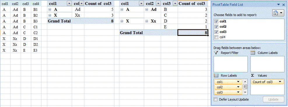
for the first table I really want to produce this

| col1 | col2 | count
+------+------+------
|  A   |  Ad  |  1
|  X   |  Xx  |  1

and the second one

| col1 | col2 | col3 | count
+------+------+------+------
|  A   |  Ad  |  B   |  1
|  A   |  Ad  |  C   |  1
|  X   |  Xx  |  D   |  1
|  X   |  Xx  |  E   |  1

So the counts reflect the distinct record count at a given level not the sum of all rows.

I need to answer questions like "what is the total of distinct items in col1"

I also need to answer this question "show count of col3 for col1"

I expect I will be asked to make graphs and present the data at various normalized levels too.

I hope this is more accurate for you. Thanks for the help so far

Peter

Posted 2013-05-23T22:26:30.477

Reputation: 111

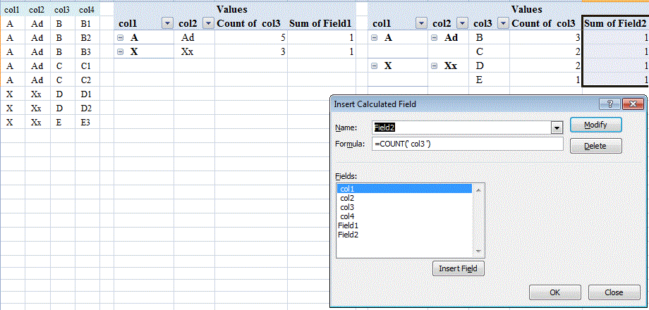
1You can use pivot table. For first result table, set col1 and col2 as row labels, set report layout to tabular form, turn off subtotals and grand total. For count of unique combinations, set values to count of column 2. Similar process for second result table, just add col3. – chuff – 2013-05-23T22:53:05.940

Answers

2

On the basis that one picture is worth a thousand words:

SU599258 example

  1. Select A:D, Insert > Tables - PivotTable, PivotTable and accept defaults (though restrict range if you do not want (blank) to appear in the results and you can't be bothered to filter it out - but then remember to increase the range if an update entails more rows. Also you could opt to include the PivotTable in the same sheet, as I have for ease of illustration.)
  2. Drag the fields to the locations shown in the PivotTable Field List example (which is for the right hand PivotTable) and ensure that values is set to Count of. (If not, left click on it and then on Value Field Settings..., select Count and OK).
  3. For the format shown I chose, having left clicked on the PivotTable, Design > Layout - Report Layout, Show in Tabular Form.
  4. If you see subtotals you don't want, right click on an instance of each of the fields involved, choose Field Settings and select None, OK.
  5. Create the second PivotTable from the first.

Note The PivotTables will not change until refreshed, though that is a simple matter of right clicking on either and selecting refresh.

Call back if you require clarification.


Edit in response to clarification of requirement

Rather than forego some analysis that might be useful even if not required at present, simply add a calculated field to each 'existing' PivotTable, eg =COUNT('col3').

updated SU599258 example

pnuts

Posted 2013-05-23T22:26:30.477

Reputation: 5 716

2

Excel has PivotTables and PivotCharts. For Excel 2007 or later, select the range containing your source data, go to the Insert tab, and choose which one you want to create. Microsoft has an overview on their website.

Nicholas Cole

Posted 2013-05-23T22:26:30.477

Reputation: 160