1
1
I'm trying to get my format sentence to work, but it just won't
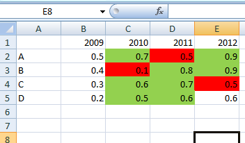
I want to format the cell green if the cell is greater than the cell before it (and that cell contains a number)
I'm trying:
=INDIRECT(ADDRESS(ROW(),COLUMN()-1))>INDIRECT(ADDRESS(ROW(),COLUMN())) AND ISNUMBER(INDIRECT(ADDRESS(ROW(),COLUMN()-1)))
I added the and because some cells with text next before them got red. It works without the AND ISNumber part

Jakob
Posted 2013-02-18T17:06:10.443
Reputation: 195


Why not something like this?
=AND(ISNUMBER($A$1),$A$2>$A$1)This will format the CellA2green if cellA1is a number andA2>A1– Siddharth Rout – 2013-02-18T17:36:00.313I'll assume that you missed my comment by mistake? – Siddharth Rout – 2013-02-18T18:03:35.037
@SiddharthRout I'm sorry, I don't see how that's different from Peter's suggestiion, only the arguments are switched, and the values are absolute and not dynamic – Jakob – 2013-02-18T18:05:52.150
I was assuming (based on your question) that there was only one cell? I see your screenshot now and understood that there is a dynamic range involved :) – Siddharth Rout – 2013-02-18T18:08:29.133
SiddharthRout - that's definitely what I want, only with dynamic cells – Jakob – 2013-02-18T18:31:15.823
See my answer below. If you remove the "$" then it becomes dynamic. – Siddharth Rout – 2013-02-18T18:32:07.973
Will it apply to all the cells in a pivot table even if the table expands beyond the range I have selected to start with? – Jakob – 2013-02-18T18:35:37.777
May I see how your pivot looks so that I can test it first before commenting? – Siddharth Rout – 2013-02-18T18:37:46.577
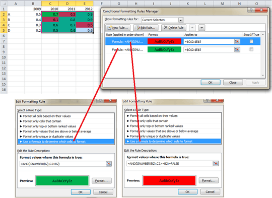
Ok after testing it on several pivots, I realized that the "Applies To" in conditional formatting remains absolute. So when the pivot rows expand all you have to do is to use the format painter to simply copy the CF to the rest of the cells. – Siddharth Rout – 2013-02-18T19:19:10.593