Formula to merge column from sheetA to sheetB to matching ID

1

Match unique id Sheet1!A2 to a cell in Sheet2!A2:A100 that has the matching ID.

Paste cell content from column Sheet2!C2:C100 from the same row with the matching id in Sheet2 to the cell with formula in it.

What is the formula for this (or how do you do this)?

The following did not work:

=VLOOKUP(Sheet1!A2,Sheet2!A2:A1000, Sheet2!C2:C1000)
kittensatplay

Posted 2012-09-11T02:31:21.160

Reputation: 217

1Your third parameter should be a number (not a range) indicating which column in the second parameter (a range) you want to access if you find a match. You should also use a 4th parameter to specify that you want an exact match or the closest match. – Mike Fitzpatrick – 2012-09-11T05:19:44.780

how will the 3rd parameter, a number, indicate "which column in the 2nd parameter" to access since a number indicates a specific cell, but i want to check the whole column. it looks like the formula in the answer is using a range, not a number – kittensatplay – 2012-10-04T18:21:28.617

Answers

1

If you would like to find the value in column C when the value in column A matches the ID in Sheet1!A2 then:

=INDEX(Sheet2!$C$2:$C$1000,MATCH(Sheet1!$A$2,Sheet2!$A$2:$A$1000,0))

user157938

Posted 2012-09-11T02:31:21.160

Reputation: 69

i opened a new excel window, pasted this code, and this made excel freeze (not responding) -- ill try again later – kittensatplay – 2012-10-04T18:33:52.920

this didnt work, a clarification is that Sheet1 or Sheet2 means a sheet within an excel window – kittensatplay – 2012-10-04T20:46:17.060

0

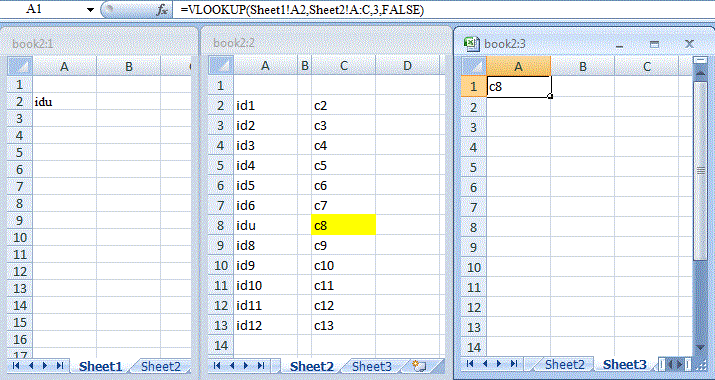
In conjunction with say a Column letter a number may indeed indicate a specific cell but the syntax for =VLOOKUP is VLOOKUP(lookup_value,table_array,col_index_num,range_lookup) (ref) so in this context a number indicates an entire column (1 for A [in this instance, since the index field is in ColumnA], so 3 for C).

A fourth parameter (range_lookup) is generally advisable (usually FALSE but 0 serves) to ensure matching of index is exact and not just 'next best'. In an array ordered ascending for lookup_value, if the fourth parameter is omitted, TRUE or 1 the formula would return the next largest value that is less than lookup_value, where there is no exact match. Where not ordered 'next best' could be almost any of the values in the (here third) column.

With FALSE or 0 the array does not need to be ordered.

It may be worth repeating that the col_index_num cannot be negative.

SU472583 example

pnuts

Posted 2012-09-11T02:31:21.160

Reputation: 5 716