Creating a chart using a dynamic named range in Excel 2010

Question

I am trying to create a scatter plot in Excel 2010 using dynamic named ranges and am having trouble getting it to work. Here's simple example that is failing:

1. Open Excel, starting a new workbook

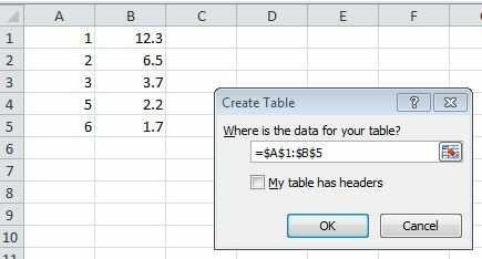
2. Enter some data:

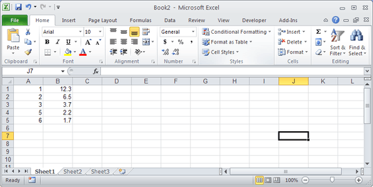
3. In cell D1, enter: $A$1:$B$5. (In my real sheet, this is dynamically computed, but manual entry still has the problem).

4. On the ribbon, click Formulas, Define Name. Define MyRange1 as a sheet-local name using =INDIRECT(Sheet1!$D$1) as shown below: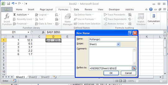

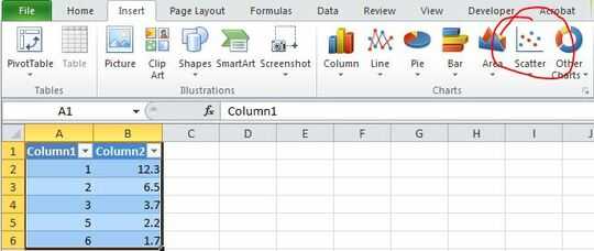
5. Click OK, and then insert a scatter chart.

6. Open the "Select Data" dialog and enter ='Sheet1'!MyRange1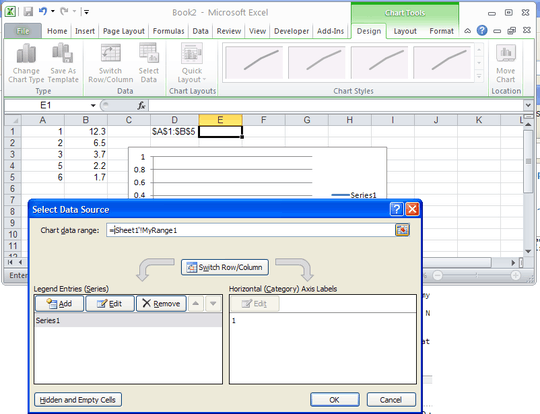

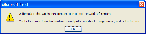
7. Excel crashes...

The problem occurs both on Windows XP and Windows 7 with Excel 2010 in both cases, repeatable every time.

---

I've also tried:

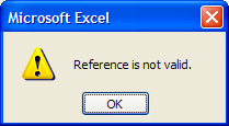
• Defining separate ranges for x and y data and using the Edit Series dialog. After entering ='Sheet1'!MyXRange in the X value field, Excel stops accepting keyboard and mouse input except for the Escape key which exits the dialog. If I go back to the dialog only then does it crash.

• Scoping the named range to the workbook instead of the worksheet. This actually does stop the crash, but I get errors in the Select Data dialog depending on whether I type =MyRange1 or ='Sheet1'!MyRange1:

---

Is this a known issue, or is there somewhere to report it? I don't have Excel 2007 or 2003 here to check if the problem is isolated to 2010. If I can't get this working I'll probably just use VBA instead of dynamic named ranges.

---

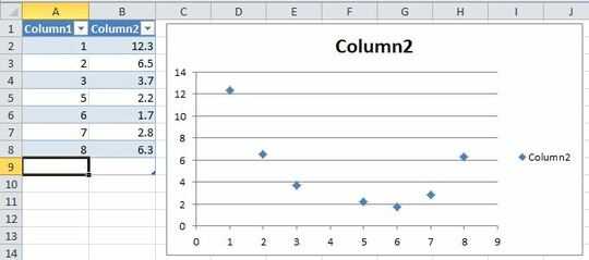
Update: I thought I figured it out (I posted an answer, now deleted). I changed the value in cell D1 = $A$1:$B$5 to D1 = 'Sheet1'!$A$1:$B$5, and the chart is created properly. However, it seems when the chart was created it is not dynamic -- it just used the current values to create the X and Y series, so changing D1 does not make the chart update.

Answer 1

1. When INDIRECT is used to define ranges, charts often don't use the ranges correctly, and often don't even accept these named ranges. There are better (more robust) ways to define dynamic ranges, using for example INDEX or OFFSET.

2. Even if the name would be recognized by the chart, it will be converted to a cell address in the Chart Data Range box of the Select Data Source dialog. Names only persist in the ranges for X, Y, and series name for each individual series.

3. If you prefix the range with the sheet name in cell D1? Charts need fully qualified ranges, so if cell D1 contains Sheet1!$A$1:$B$5 you can use your defined name in the Chart Data Range box of the Select Data Source dialog. Note that, per point 2, Excel will convert this range to its cell address when you click OK.

Answer 2

According to the link below and my personal testing of it, you must enter the data series in the form of

'WorkbookName.xls'!RangeNameX

If your name is dynamic, then the resulting chart will be too. The formula I used for my dynamic named range was (modify for your situation and use for both X and Y ranges).

=OFFSET($A$1,0,0,MATCH(1E+306,$A:$A,1),1)

That worked to make the chart dynamic as far as adding newly appended values to the chart (required both X and Y values before chart updated).

Source for how to Setup Chart - Microsoft Q&A Site Source for hot to use Dynamic Ranges - OZGrid

Answer 3

Here is how I create a dynamic chart.

1. Create a table from your data.

   

2. Highlight the table
3. Go to the insert tab and select the type of chart you want.

When you add data to the table, it will be updated to the chart as well.