4
I'm using Excel 2010 and would like to know if there's any way I can choose conditional formatting to highlight only instances of duplicates when it's found in ALL the columns I chose?
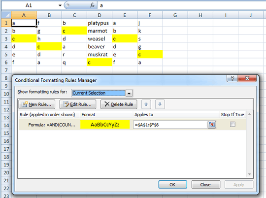
For instance, I have six columns of data, with duplicates in them, but I only want those duplicates to be highlighted if they appear in ALL SIX columns.
E.g.
Column A Dog Cat Fish Horse Platypus
Column B Cat Platypus Panda Chicken Dog
Column C Bird Zebra Giraffe Platypus Panda
Column D Platypus Bird Dog Zebra Horse
Column E Otter Lion Platypus Giraffe Zebra
Column F Lion Ostrich Platypus Dog Snake
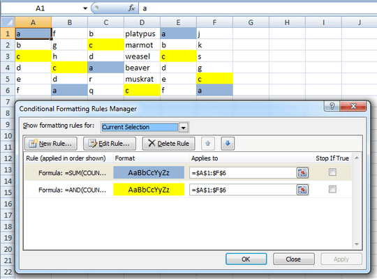
Only "Platypus" appears in all six columns, but "Dog", "Cat", "Horse", etc all have one or more duplicates, which will usually end up being highlighted. If I can find a solution that will allow me to have the flexibility of choosing to highlight instances of duplicates in 5 out of 6 columns, 4 out of 6 columns, 3 out of 6 columns, etc, that'd be even better!
Note that the data is not arranged nicely in a row, so that I couldn't use "Countif" across rows to see how many times "dog" appeared in Column A-L on a specific row (i.e. "dog" could appear anywhere in the columns, not necessarily on the same row).
If anyone has any tips on this, I'd really appreciate it, thanks!!

C. Y Y
Posted 2012-08-09T14:00:15.727
Reputation: 43

Hi Excellll, am I understanding your formula correctly that it means I must first manually identify the values that are duplicates (i.e. the A1 you have in your formula) and then plug it into the conditional formatting rule? – C. Y Y – 2012-08-09T15:27:07.993
1@C.YY No, not at all.
A1is just the top-left cell in the range you're applying the rule to. SinceA1is a relative reference, the rule will apply to each cell in the range, withA1replaced by the address of each cell. I.e., the rule applied toB2will be the formula with all instances ofA1changed toB2. This is done automatically -- one rule should find them all. – Excellll – 2012-08-09T16:30:07.4601In case that isn't clear, the key is that formulas for conditional formatting are written to apply to the top-left cell of the target range. The formula is applied to each other cell as if it is being filled down and across the range. That is, the relative cell references are offset, and fixed references stay the same. – Excellll – 2012-08-09T16:33:36.443
Oh I see, that makes a lot of sense. Thank you soooo much for the help, you saved me hours of staring at the screen (and the potentially errors with that). Thanks a lot also for the detailed explanation and examples, you're awesome! – C. Y Y – 2012-08-10T16:59:01.810
Hi Excellll, actually I have another question now...I went through my data set and managed to highlight all the duplicates I wanted to, but now I'd like to essentially "count the formatted cases" i.e. determine how many values appeared in all 6columns, all 5 etc. I know using the formula you gave would be a good start, but the value always turns out "FALSE". What am I doing wrong? – C. Y Y – 2012-08-10T20:33:12.543
@C.YY I advise you to go ahead and post this as a separate new question. It's best to avoid having new questions and answers buried in the comments. That way, the site will be maximally useful (i.e., searchable) for visitors with similar problems. – Excellll – 2012-08-10T20:56:50.610
This answer was very helpful! But (at least for me) in order to run it i had to change the "," at the script with ";"... – Machine – 2013-03-15T14:09:38.603