Excel: Find rows with first column empty

0

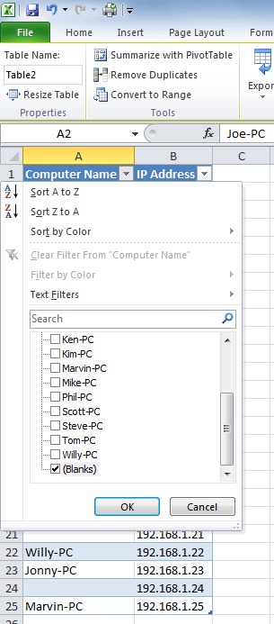
My company uses a giant excel spreadsheet that shows which IP Addresses are being used by which computers (among other information). IP Addresses that are not in use still have a row, but the computer name field will be empty.

Lets say, for example, that my spreadsheet might look like this:

Computer Name  |  IP Address  
---------------+---------------  
Joe-PC         |  192.168.1.2  
---------------+---------------  
Tom-PC         |  192.168.1.3  
---------------+---------------  
               |  192.168.1.4  <----- This IP is not used
---------------+---------------  
Scott-PC       |  192.168.1.5
---------------+---------------

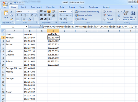
I would like to create a list of all the IP addresses that are currently not in use. So, I need to search for all the rows where "A" is empty, and then add "B" to the list. Is there a way to do this within excel?

jwegner

Posted 2012-02-08T15:59:06.173

Reputation: 178

Please [edit] your question with the version of Excel you are using. This will help get a more precise answer to your question. – CharlieRB – 2012-02-08T16:11:23.780

Answers

2

In 2010 make a insert a table and check the "My table has headers" box. It should have selected all the data. If not, enter the correct range then click OK.

Once the table is created, click the filter button on the "Computer Name" header. Unselect the check box for "Select All" and scroll to the bottom and select "Blank". Click OK and it will only show you the rows without a computer name.

enter image description here

Once you have this data, if you want to transfer it to another column/sheet/workbook, select your range and hit alt+; to select only visible cells and hit ctrl+c to copy the selected visible cells.

If you are using a previous version, these specific instructions may not work.

CharlieRB

Posted 2012-02-08T15:59:06.173

Reputation: 21 303

1This works in 2007 and in 2003 it's called a list and still works. – Jesse – 2012-02-08T17:20:20.460

+1 You are absolutely correct. I believe the way to accomplish it is quite different than 2010 though. – CharlieRB – 2012-02-08T17:58:05.867

0

This macro will paste your list in column C

Sub AutofilterBlanks()`

    Columns("A:B").Select
    Selection.AutoFilter
    ActiveSheet.Range("A:B").AutoFilter Field:=1, Criteria1:="="
    Columns("B:B").Select
    Selection.SpecialCells(xlCellTypeVisible).Select
    Selection.Copy
    Range("C1").Select
    ActiveSheet.Paste
    Application.CutCopyMode = False
    Selection.AutoFilter

End Sub

Raystafarian

Posted 2012-02-08T15:59:06.173

Reputation: 20 384

0

You can create the list with an array formula:

=IFERROR(INDEX($B$1:$B$20,SMALL(IF($A$1:$A$20="",ROW($B$1:$B$20)),ROW()-1)),"")

Enter by pressing Ctrl+Shift+Enter. Then, fill down as far as you need to.

enter image description here

It's worth noting that this is a dynamic solution; when your table is updated, the list of available IP addresses will update too with no user input. Just make sure your formula is filled down sufficiently far.

Excellll

Posted 2012-02-08T15:59:06.173

Reputation: 11 857