Can I group all rows with a percentage of column total less than 1% in an Excel 2010 pivot table?

1

This is how my data looks right now, based on hours of work logged per project in 2011:

Proj. Hrs %
A     15.6%
C     7.3&
...
X     6.1%
D     5.3%
Q     1.8%
F     1.6%
H     0.7%
Total 100%

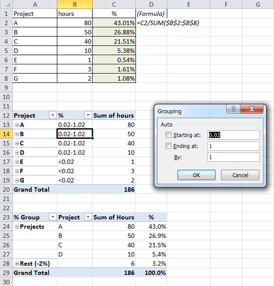
I would like to group smaller projects into a single entry, where a smaller project is one that I have booked less than 2% of my hours on.

Proj. Hrs %
A     15.6%
C     7.3&
...
X     6.1%
D     5.3%
Rest  4.1% <<< Group of all proj < 2% with total % for all combined
Total 100%

How can I do that? Do I have to change the data before I make the pivot table, or can I do it with the pivot table I have already?

Michiel van Oosterhout

Posted 2011-12-30T21:34:42.413

Reputation: 658

Answers

2

1) First, you can do it manually by creating a group on your Project row label. Just select projects under 2%, and right-click Group By.

2) Second, if you want something more dynamic, one way to do with would be to create a Group Field on a % row label on your pivot table. Unfortunately this requires that the % column comes from your source data since a Pivot Table cannot group its own summarized values.

So adding a formula to calculate the % in your source data would allow this method to work, as shown below. One group will be called >2% and be left expanded, while the <2% group will be collapsed.

enter image description here

If calculating % in your source data is too cumbersome, another option is to create a pivot table on an intermediary pivot table, but that can bring a new set of issues.

mtone

Posted 2011-12-30T21:34:42.413

Reputation: 11 230

I'm facing exactly the same problem. Could you please describe how to build Pivot Table for this case. – madhead – 2014-05-29T08:07:55.957

2

You are going to have to do the summation group BEFORE you go to the pivot table.

Probably the simplest way to make this work would be to use a sumif formula - like this:
=SUMIF(C5:C15,"<=0.02",C5:C15)

That will give you a single cell with anything = to or less than 2%. Use an IF function to filter your percentages in a new column. Using your examples, like this:
=IF(C5>0.02,C5,0)

So now your source range looks like:

Proj.    Hrs %        Hrs2%
A        15.60%       15.6%     (these are IF statements.)
C        7.30%        7.3%
X        6.10%        6.1%
D        5.30%        5.3%
Q        1.80%        0.0%
F        1.60%        0.0%
H        0.70%        0.0%
B        24.20%       24.2%
M        15.00%       15.0%
J        20.40%       20.4%
p        2.00%        0.0%

Rest                  6.1%  (this is the sumif statement)

Set the pivot table to include the "Rest" row in the source data range, and the filter not to show 0 values in the pivot table.

You may have to play with it some - the natural sort will show your "rest" where the value is. In the data above, "Rest" after everything except project X, which also has a 6.1% value. You could jigger your naming convention to work around that.

corvus

Posted 2011-12-30T21:34:42.413

Reputation: 41