Text values in a pivot table?

Question

I have a table (in MySQL) with 3 columns:

Location    Category     Supplier

   A        Computers    Company X
   A        Printers     Company Y
   B        Computers    Company X
   B        Printers     Company Y
   B        Software     Company Y
   C        Computers    Company Y
   C        Software     Company Z

Now I need to make a matrix containing the above information , like this :

       Computers      Printers       Software

A      Company X      Company Y
B      Company X      Company Y      Company Y
C      Company Y                     Company Z

Eventually I need to have this in Excel.

In reality I have a variable number of categories, so doing it in MySQL with a join for each column is not a good option. I could write a function in PHP, but I was wondering if there's a more elegant solution.

I looked a pivot tables in Excel, but they seem only suited for numbers as values. But maybe I'm overlooking something, since I never work with Excel myself.

Answer 1

I don't know if this is as "elegant" as you were hoping for, but you are on the right track with the pivot table idea. You just have to cheat a bit. A "helper column", a pivot table, and the "vlookup" function can be your friends here.

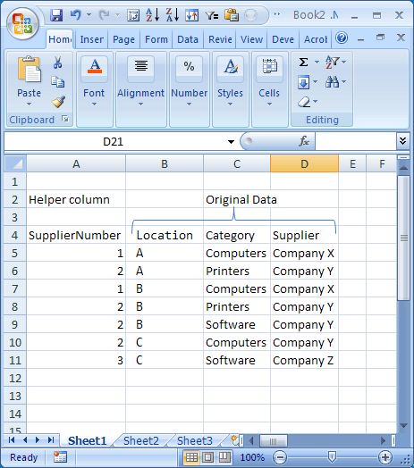
First, to the original data, add a helper column for a "SupplierNumber". Company X = 1, Company Y=2, Company Z=3. I put the helper column as the first column, for easy use later in a vlookup. Note the data is now in cells A5:D11.

Next, pivot the data like this. I used the "classic Pivot table layout" option in the "Display" tab of the "Pivot Table Options" dialog (right-click on the pivot table to bring that dialog up).

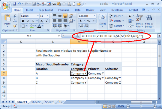
Select and copy the entire pivot table, then "paste special/values" in another location to the side of the original pivot table. Then, in the body of the table copy, enter the formula shown. Note that the vlookup formula is referring back to the original pivot table (the "H7" reference -- see the previous diagram) and also to the range A5:D11 mentioned earlier.

Like I said, it's not elegant, but it works. There are a lot of smart people that browse this site who will likely come up with an "elegant" solution for you!

Answer 2

I figured out that you can avoid the pivot table altogether. See the screenshot below. Use a helper column. Define the named ranges shown. Set up your layout as in G14:J18. In the body of the table, use VLOOKUP with a SUMPRODUCT.