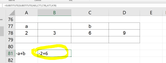
You could use the following and adapt as required for choosing the lookup values. (For example, you might have 10 variables, not just "a" and "b".) You might also need to adapt for operators and the negative sign if other expressions need evaluated.
=-HLOOKUP("a",$A$77:$D$78,2,FALSE)+HLOOKUP("b",$A$77:$D$78,2,FALSE)
The above is the simple version assuming that exact set of variables and that exact expression.
A note of interest for you since you indicate you sought a solution with `EVALUATE()~. You DO have access to that formula. Where you are running into trouble is that it does NOT work "cell-side" (in the open spreadsheet. It is only available in the Named Range functionality.
The idea would be for you to make a Named Range, perhaps "Answer", and use this formula in the "Refers to" box:
=EVALUATE(-a+b)
You would need to EITHER replace the "a" and "b" in that with the corresponding portions of the formula from above, of define them as Named Ranges themselves. I prefer the latter personally, though some single letters, "c" for example, are not available (it conflicts with the "C" in the R1C1 addressing style; so does "r"). You could give the Named Ranges names like "AA" and so on, using SUBSTITUTE() for the raw input from the cell. Or just the ones Excel won't let you use directly.
The important element of this, since my wager is that you found an EVALUATE() solution elsewhere and just need to make it work, is:
EVALUATE() MUST BE USED IN NAMED RANGES OR IT WILL NOT WORK. And EVERYONE can use it, not just some, so long as they use it inside the Named Range functionality.
All the old Excel 4 macros are available that way: in Named Ranges, never, ever, in the cells of the spreadsheet itself.


2
Does this answer your question? Excel function that evaluates a string as if it were a formula?
– Akina – 2020-02-10T08:09:48.260If your problem is this much only then better assign NAME to cell A78 & C78 then use both to Add!! – Rajesh S – 2020-02-10T08:48:01.417
@Akina no, I tried that before asking and I did mention that evaluate not exist. – anhnha – 2020-02-10T09:17:40.090
@RajeshS I have a lot of expression and need to use substitute – anhnha – 2020-02-10T09:19:00.767
evaluateExists in VBA in all versions of Excel – Máté Juhász – 2020-02-10T15:26:06.977