MS EXCEL: How to make changes in tabs show on Master

0

This is such a common question I feel a bit stupid asking it! Master sheet has a list of kids names and their classes. The tabs are different classes. There is a column to check attendance; 0 for no-show 1 for present. Once checked this will show on attendance column on Master - remember there are about 10 tabs. I want something simple like =Class1! but how do I get this to work? An IF would also work but which is easier, especially if kids change class. It is baffling me!

enter image description here

Garry Smout

Posted 2019-05-02T03:09:29.743

Reputation: 1

1Its hard to understand what you are trying to achieve. I am going to assume that you are trying to do some sort of lookup - using kids names and class, go to the corresponding class tab, look for the kids name and grab the attendance value from one of the columns. Is this correct? – Bharat Anand – 2019-05-02T03:18:03.667

If this is what you are trying to achieve, it can be done using INDIRECT() function. Ref: http://spreadsheetpro.net/how-to-make-a-dynamic-reference-to-a-worksheet-in-excel-and-google-spreadsheets/

– Bharat Anand – 2019-05-02T03:27:40.640

'Once checked this will show on attendance column on Master' this does not describe your need. "this" will "show" what? How many columns are there on Master sheet? What do they describe? 'something simple like =Class1!' can be accomplished by typing = then clicking into the sheet called Class1 and selecting the cell you wish to reference. – Alex M – 2019-05-02T07:21:14.030

Answers

2

Below answer is based upon the assumptions I have laid out in the comments to your question.

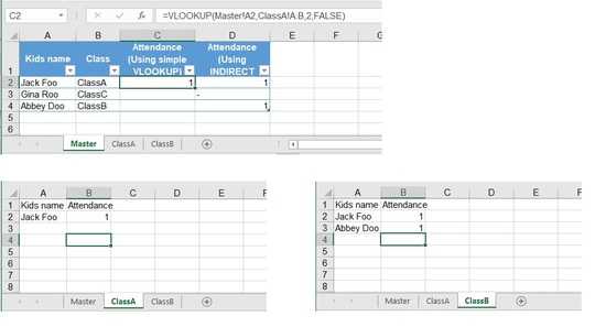
A regular way to reference the attendance information would be using VLOOKUP (if the sheet where you need to lookup is known) as below:

=VLOOKUP(Master!A2,ClassA!A:B,2,FALSE)

However, since the lookup sheet needs to change based upon the Class column on your Master sheet, so use an INDIRECT function to refer to the sheet name stored in this column. Usage will be as below: =IFERROR(VLOOKUP(Master!A2,INDIRECT("'"&B2&"'!A:B"),2,FALSE),"-")

Reference sheets setup as per the pic below: enter image description here

Bharat Anand

Posted 2019-05-02T03:09:29.743

Reputation: 346

No, this is not what I am after. In the tab a teacher puts a 1 or a 0 in the column (once checked) and this is shown in the master sheet so a principal can see ALL the classes attendance in one sheet. IF works but needs to be nested and having problems with that, and so should CLASS1! CLASS2! but that also has problems. What is needed is so simple I just can't understand how complex it becomes! – Garry Smout – 2019-05-02T03:57:17.347

1I'm sorry but you need to write a little bit more clearly. The example that I have shown here is based upon the minimal inputs that you have provided. This is designed so that the inputs in ClassA and ClassB tabs will aggregate (or show up) in the Master tab. Based upon what you have written, I believe this is what you are after, if not then please update your problems with some sample images and the formula that you are using and where it is not working. Only then the StackExchange group will be able to help you meaningfully. – Bharat Anand – 2019-05-02T04:42:10.980

Thanks. VLOOKUP has some of the answers and INDIRECT gets round the VL problem - better than Nested IF. There will be over 10 classrooms with 3 attendance checks per day, so gets quite complex and because I don't know the two methods you demonstrate above I am a bit hesitant to try them out! That " ' " for example! – Garry Smout – 2019-05-02T07:15:22.670

@GarrySmout Can you just edit your question to clearly state what you have and what you need? It's not necessary to state that it's complex. Show a sample of what it should look like. – Alex M – 2019-05-02T07:18:29.737

@GarrySmout, thanks for sharing the screenshots. I understand your frustration, getting started with SE (stackexchange) can be a bit daunting, but is rewarding in longer run. Now we have some idea of your problem. You seem to be using an existing excel designed by someone prior to you, and are trying to make this attendance tracker smarter. If so, in all probability you might be heading for a major re-write of this solution and will require a good handle on using VLOOKUP function. Current excel solution appears to be a hard-coded sheet. Have patience and good luck! – Bharat Anand – 2019-05-02T23:53:19.890

0

You can do this using xl queries. Ensure that the data for each class on each tab are formatted as a table. All the tables must have EXACTLY the same headers. Beware spelling and stray whitespace.

Go to your first class data tab and select the top left cell. From the Data menu tab, Get & Transform item select 'From Table'. This will pop up the query editor. Go to the 'Close & Load' dropdown on the left, select 'Close and Load To ...' then select 'Only Create Connection'. Click Load. Do this for each Class tab.

Then from Data\Get & Transform select 'New Query', goto Combine Queries and select 'Append' .

A pop up appears asking if it is a two table or three or more table append. Three or more in your case I guess. Using the 'Add 》' button add all class tables to the 'Tables to append' box. Then select OK.

The Power Query editor will popup with a preview of the whole dataset.

Again select 'Close & Load To ...'

In the Load dialog leave 'Table' selected. Select 'Existing Worksheet:' Navigate to your Master sheet and select the location you want.

Click load. Voila.

This is a sortable filterable table. Update with the Refresh All button on the Data menu tab or the Query dynamic menu tab.

Excel queries can be a bit of a rabbit hole but consistent table design / db structure will help & there are plenty of resources out there.

PS this will pull in ALL the data from the Class tables. You can limit that in the individual class queries or the final append but that is a separate question.

Good luck.
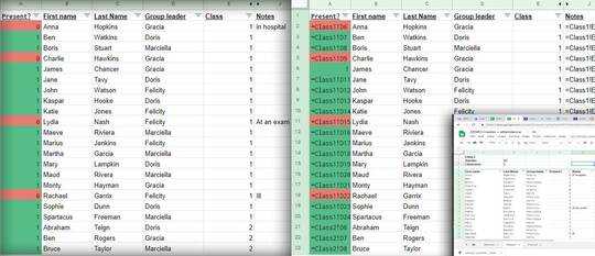
pHred

Posted 2019-05-02T03:09:29.743

Reputation: 101

0

Since you have not provide sample data so on the basis of prices information with the question, I've created this solution which reflects Attendance Status on Mater Sheet, using records from Class Tabs.


enter image description here


enter image description here


enter image description here


How it works:

Formula in Master Sheet:

  • In Cell C4 to get attendance of Class I,

=IF(ISBLANK(ClassI!C3),"",IF(ClassI!C3=0,"Ab","Pr"))

  • In Cell C7 to get attendance of Class II,

=IF(ISBLANK(ClassII!C3),"",IF(ClassII!C3=0,"Ab","Pr"))

  • Fill the Formula Right then Down.
  • Adjust Records on Sheets & Cell references in the Formula as needed.

Rajesh S

Posted 2019-05-02T03:09:29.743

Reputation: 6 800

Thanks. This is close to what I imagined but with over ten classrooms and 400 students - who might change rooms - and 3 attendance checks per day, I will need nested IFs and I think that is impracticable. Going to try with IFS and if that fails will take a look at look at Bharat's solution. – Garry Smout – 2019-05-02T07:21:25.063

@GarrySmout,, you are already creating Tabs for Classes and the Master Sheet,, now what is required use the Formula in Master Sheet and Fill among required Rage also,, even attendance has not been filled in Class Tabs,,, Formula will return BLANK and as soon you fill attendance you start getting RESULTS on Master sheet ,, you can escape from Data Entry !! – Rajesh S – 2019-05-02T07:30:49.477

How do I post an image of a spreadsheet that is similar to one we used last year. It just uses =Class1!D7 etc but I can't seem to re-create this ... and @Rajesh S I think I understand but a little more detail would be fantastic! Everybody asks me to be 'clear' and I honestly can't be clearer: You write something next to a name in a tab and it appears in the Master, next to same name! – Garry Smout – 2019-05-02T08:33:21.040

@GarrySmout,, below your post you find small row of links, there you find Edit click it, then either Copy & Paste part of Sheet or Copy required portion & Paste in Paint Brush, or use Print Screen then Save the portion in Paint brush file, finally on top of editor you find IMAGE Icon click and follow the instruction. – Rajesh S – 2019-05-02T08:59:02.703

Thanks @Rajesh S. Can't post images just yet but the word 'NAMES' in original post is now a link. – Garry Smout – 2019-05-02T09:13:13.713

@GarrySmout,, is almost similar what I've used as example,, mine is technically better you have tried to link cells between sheets using =TABName!Cell addres, once try what I shown!! – Rajesh S – 2019-05-02T09:41:15.157

Will try your way as I can't get IFS to work. – Garry Smout – 2019-05-02T10:43:56.907

Can get just one Class Tab) to show and work in Master. To add data from a second tab I get Inconsistent calculated column formula warning. I have an empty, clean line between classes in Master, but I guess it is still 'column'. I am creating the formula - =IF(ISBLANK(LEVEL1I!F2),"",IF(LEVEL1!F2=1,"P","AB")) =IF(ISBLANK(LEVEL2!H4),"",IF(LEVEL2!H4=1,"P","AB")) – Garry Smout – 2019-05-04T03:33:04.937

overran edit time! First formula above is H2 not F2. I also filled in all of cells with formula before doing second. Should formula be done to each pertinent cell then filled in, as implied in your example? – Garry Smout – 2019-05-04T03:44:18.993

I seem not to have mastered the art of adding a name, the two comments above were for @Rajesh S. – Garry Smout – 2019-05-04T03:46:43.140

@GarrySmout,, yeah in above comments the Formula you have shown is correct, what you need to do is,, Copy the Formula either after or even before you enter attendance in Class TABs and fill across column,, as soon you enter attendance in Class TAB you get Attendance status in Master Sheet.. follow instructions I've written with my post, you achieve it easily !! – Rajesh S – 2019-05-04T06:10:32.763

Thanks @Rajesh S. It seems to work if Master is NOT a table. Keeping it simple does the job! – Garry Smout – 2019-05-04T06:33:03.040

@GarrySmout,, formula will work for both Table and Simple Data Range,, better try on Simple Data Range First, then on Table ,, if you find that my solutions works for you then you may accept it as answer as well up vote also! – Rajesh S – 2019-05-04T06:41:18.810