1
I am creating a list of features and the audiences that will be targeted for those features. Each stakeholder group (audience) is separate by a comma in the list. Now, if I want to create a pivot or some formula to see which features are applicable for a particular stakeholder group, then how would I do that.
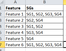
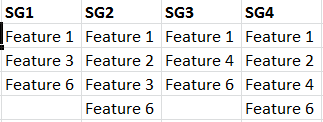
In the image above, the table has the features listed vertically, and each feature has a list of SGs (stakeholder groups) assigned to it. Now, I want another table in where I can select any particular SG, and it will return the features this SG is mapped against. Here is the expected outcome:
Is there a way to do this?


Since SGs are duplicate therefor will return multiple Features, this is what you are suppose to do or anything else,, better edit the post and attach expected output also !! – Rajesh S – 2019-04-09T05:08:58.167
@RajeshS I added sample output – JayD – 2019-04-09T16:08:11.787
If you have a reasonable number of features and SGs, and you don't NEED the output of the vertical feature list to roll up without interstitial blanks,
=IF(ISERROR(FIND(D$1,$B2)),"",$A2)copied from the first cell under SG1 across the entire sample output table will work (assuming SG1 is inD1) – Alex M – 2019-04-09T18:34:47.863@JayD,, now check the post I've solved the issue!! – Rajesh S – 2019-04-11T05:55:51.940