Lookup functions, like VLOOKUP or the combination of INDEX and MATCH, are very common, basic functions used in Excel, so it's worth getting familiar with them. To get you started, there's a good explanation of VLOOKUP here.
Here's the gist using your example:
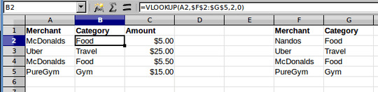
Some made-up data is in columns A and C. In another spot on the worksheet, or another worksheet, you have the lookup table. I stuck it in columns F and G. Column B is where you want to fill in the category for each entry. The formula in B2 is:
=VLOOKUP(A2,$F$2:$G$5,2,0)
You just copy it as needed. The reference to the merchant in column A isn't anchored, so that will reflect the current row when you copy the formula down the page. The lookup table in F:G is anchored with absolute addressing (the dollar signs), so it will continue to point to the table when you copy the formula. The third parameter tells VLOOKUP to retrieve the result from the second column of the table. The last parameter (0 or false), tells VLOOKUP to do an exact match on the merchant name.
Enhanced Solution
You presented a challenge in your comment, suppose the merchant entry in column A is a random text string that contains the merchant name in the lookup table. You could do that with something like this:
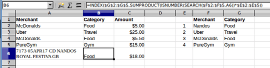
In row 6, I added the example in your comment. I also added sequential numbers for the table rows next to the merchant name in the lookup table. The formula in column B (shown for B6 in the formula window):
=INDEX($G$2:$G$5,SUMPRODUCT(ISNUMBER(SEARCH($F$2:$F$5,A6))*$E$2:$E$5))
This uses INDEX to pull the category from column G based on the table row produced by the SUMPRODUCT.
SUMPRODUCT lets you do array operations on a range. It uses the SEARCH function to see if each merchant name in column F is contained in the merchant string in column A. Search returns a position or an error, but we're only interested in whether it's there, which would be a numerical result. ISNUMBER returns a 1 for true or 0 for false, which is multiplied by the table row number added in column E. The result of the SUMPRODUCT will be the table row of the matching merchant.
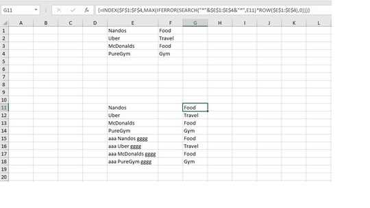
If you want to make the merchant name more visible, you could insert a column to the right of A to display just the merchant name as stored in the lookup table. You could use the same formula as above for that, but have the INDEX range point to column F instead of column G.


The typical way to do this is to create a lookup table with the merchants and their category. In col B, you would use VLOOKUP or INDEX+MATCH to look up the merchant in the table and return the category. – fixer1234 – 2019-01-16T10:01:24.247
Sounds like it would work for sure, can you give me more explicit instructions, I'm a relative beginner :) – Jason Broderick – 2019-01-16T10:04:11.510
Welcome to Super User. I posted an answer for you, but just a heads up, the site encourages people to do a little research before asking questions. Questions that are basically, "This is what I need; do the work for me and hand me an answer", aren't well-received. You'll typically get comments like, "What have you tried" or "Super User isn't a free coding service". So you'll know for next time. :-) – fixer1234 – 2019-01-16T10:43:08.827