Identifying different permutations of some field in Excel holding others constant

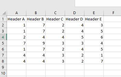
In Excel 2016, I have a worksheet with five columns of headings (A through E) and many rows of data. I'm trying to find entries that have the same data for columns A through D and to identify what the different versions of the data in column E are given the data in A through D.

So far I have created a pivot table that has columns A through D as rows and the distinct count of E is shown as the value. This allows me to see which combinations of A through D have more than one possible E value but I'm not sure how to retrieve what those values of E actually are.

In the end I would like to populate a separate worksheet with all the possible A-D combinations paired with all of their possible E values. Is this possible to do with a pivot table or would I need VBA? Should I consider a different approach?

Any help is appreciated. I've attached an example screenshot which may make my problem statement more clear. In the example the first two rows would have the same A-D values and the possible E values would be 3 and 5.

Kyle Jones

Posted 2018-06-12T13:20:12.380

Reputation: 107

Are the values in A,B,C,D enumerable within their columns? i.e. if you have color in A, fruit in B, price in C, store in D? or might you have the same value in A as you might find in B? Is their order important? – JaredT – 2018-06-12T13:28:00.630

columns A,B,C,D all indicate different things as in your first statement (color for A, fruit in B, etc). – Kyle Jones – 2018-06-12T13:30:33.263

Answers

I am just expanding on JaredT's great idea.

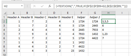
In F2 enter:

=TEXTJOIN("",TRUE,A2:D2)

and copy downward.(use concatenate if you don't have textjoin). Then copy column F and PasteSpecialValues into column G.

Then remove duplicates from column G

We can now gather all the column E items associated with cols A through D. In H2 enter the array formula:

=TEXTJOIN(",",TRUE,IF($F$2:$F$99=G2,$E$2:$E$99,""))

and copy downward:

EDIT#1:

This is an array formula. Array formulas must be entered with Ctrl + Shift + Enter rather than just the Enter key. If this is done correctly, the formula will appear with curly braces around it in the Formula Bar.

Gary's Student

Posted 2018-06-12T13:20:12.380

Reputation: 15 540

This looks to be exactly what I want to do. However when I copy the exact formulas and test file in your example, row H does not do what your screen shows. There doesn't seem to be a way to attach a picture to a comment but H2 contains all values of E separated by commas and the rest of H remains blank. Any idea why that is? When I created row G I simply copy and pasted values and then did a remove duplicates under the Data tab. – Kyle Jones – 2018-06-12T14:41:03.307

@KyleJones My error, not yours ...........see my EDIT#1 – Gary's Student – 2018-06-12T15:03:03.017

You did mention it was an array formula, thanks you've been very helpful! – Kyle Jones – 2018-06-12T15:05:45.427

1That's why I always show array-entered formulas with the braces surrounding them. That's a visual reminder when you copy-paste that you need to remove them and array-enter the formula. – robinCTS – 2018-06-12T15:09:36.727

@robinCTS Very good idea! I usually show the braces in the picture and include the instructions in the text. I forgot the text this time. – Gary's Student – 2018-06-12T15:12:49.253

A simple solution

The simplest, if perhaps the ugliest, option is to add a helper column, maybe call it group, which is just a concatenation of columns A->D; e.g. =CONCATENATE(A2,B2,C2,D2) which may leave you with a value of RedApple$1PigglyWiggly. Obviously you can add delimiters to make it easier on the eyes. It would be a simple operation to group on this field in your pivot table.

JaredT

Posted 2018-06-12T13:20:12.380

Reputation: 1 012

Thank you, this is a good idea. After I've done this how would I go about identifying each possible E value for each of my group entries? – Kyle Jones – 2018-06-12T14:46:23.113