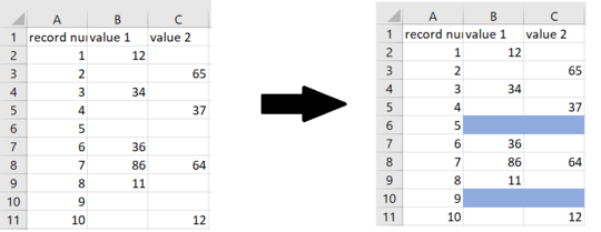
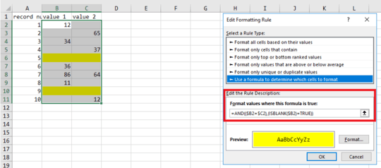
How to highlight blank cells in a row only when both adjacent cells in the row are blank?

Question

I'm looking at two columns and if a row has blank cells in both columns, I want to highlight both blank cells (but nothing would be highlighted unless both are empty). How can I do that?

Answer 1

Apply the formula Conditional Formatting to range B2:C11

Formula is: =AND(($B2=$C2),(ISBLANK($B2)=TRUE))

Answer 2

When you encounter an Excel problem that seems complex, break it down into the components that need to be accomplished.

1. You need a conditional statement to control the formatting in each cell.
2. You need to test for blank cells.
3. The condition test needs to evaluate both adjacent cells.

Let's start with #2, testing for blank cells. There are lots of methods. A few commonly used ones are shown in columns E:G below (what is shown in the header is just the test, not an actual formula):

You can use any test you want, just pick the one you prefer.

The next step is testing that both cells meet the condition. There are lots of ways to do this, also. You can evaluate each cell and then look at the combination of results. Here are some ways to do that:

Column J uses the AND function to test whether both individual tests are true. Columns K and L use Boolean arithmetic, based on TRUE being treated as a value of 1 and FALSE as a value of 0.

When you're testing for blanks, you can test whether multiple cells are blank using the fact that stacking blanks next to each other still results in a blank. You can concatenate the cells with an ampersand.

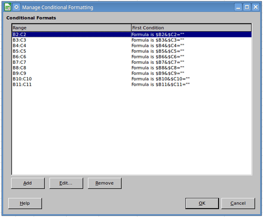
So you have a bunch of different ways to do the test. You just need to select one and use it in a conditional formatting formula. I'm using LibreOffice Calc, so the user interface is a little different from Excel. But what I used for my example is this:

I set up the first row and then used Copy and Paste Special, Formats to replicate the conditional formatting to the other rows.