Excel text + numerical sorting?

I've searched around already and couldn't find an answer to this -- pardon if it's been asked and answered already!

I've attached a photo to illustrate the dilemma. So I've sorted the data by call #, title, then serial #, but the volumes aren't sorting properly (i.e, vol. 1, vol. 10, vol. 2, vol. 20, etc.). I think it's because Excel is reading the data as text instead of numbers. Short of getting rid of the "vol." before the integers (I have over 9000 rows!!!), is there a way to sort this properly?

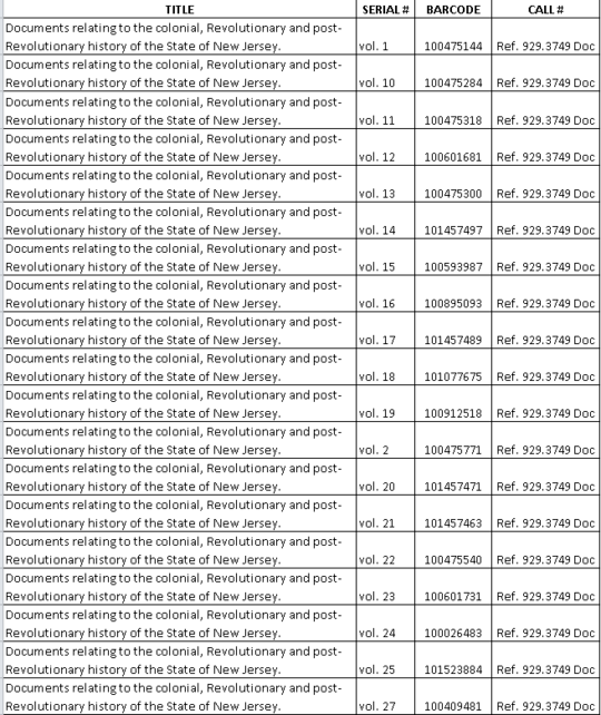
My data:

funkydodel

Posted 2017-09-09T00:03:10.220

Reputation: 11

3You will need to parse the string into a new column that only has the number or parse the string in a new column and make the number part a 2 or 3 digit number vol. 001, vol. 002,... and copy it back. – Scott Craner – 2017-09-09T00:10:45.457

Answers

Another method -- one I happen to personally prefer for this scenario of usage -- is to simply input Column B cells as numerical values only, then apply custom formatting (Ctrl+1, Tab, End, Tab) as "Vol. "##0. This way your cell data retain their numerical data type, but visually output the prefix desired.

EDIT: To fix your existing column, you could use the other suggested methods to first remove the text portion, then copy & paste-as-value the results back over the original column to overwrite it with the number values only (apply formatting after that).

Arctiic

Posted 2017-09-09T00:03:10.220

Reputation: 406

Or just use Ctrl+H and replace "vol. " by "" – Ola Ström – 2020-02-16T11:11:21.177

@OlaStröm I was referring to that by ...the other suggested methods..., but using Ctrl + H alone would still leave the cell format as Text, whereas Paste-As-Value will reset the formatting back to General, which would resolve the OP's issue.

However, I just noticed that the Ctrl + H prompt includes an option to designate the replacement content's data formatting, which would work just as well. – Arctiic – 2020-02-16T13:30:34.020

Two easy ways to do this:

Ctrl+H replace "Vol." by 'empty' and turn the result onto numbers and then sort, if the data is not dynamic and you don't care for "Vol."
Create another column between serial number and barcode with the formula: =mid(B2;5;5)*1 and then sort by this new column. Better for dynamic data when you're always adding rows.
If the number you're interested in goes from 0 to 999 and it's always at the back of the cell, you could also use =TRIM(RIGHT(B2;3))*1 instead.

Fernando Eblagon

Posted 2017-09-09T00:03:10.220

Reputation: 71

I tried option 2, but it didn't work. I was supposed to drag that formula all the way to the end, right? Also, what exactly does the formula do? Just curious! – funkydodel – 2017-09-13T00:33:24.320

I think I just need to get rid of the "vol." or add zeroes to make the three-digit numbers. Problem is, I have data like "2007 vol. 10," so getting rid of the "vol." wouldn't help much, right? – funkydodel – 2017-09-13T00:39:46.667

For option 2, the formula needed to get dragged down, not to the right. Maybe my answer wasn't as clear. I'll edit for clarity.

If you have something like "2007 vol. 10" and the numbers go from 1 to 999, you can replace =mid(b2;5;5)1 by =left(b2;3)1 since this will be better at handling additional data at the beggining of the cell. – Fernando Eblagon – 2017-09-13T13:54:06.663

Sorry, =RIGHT(B2;3) not left(...), the answer has a better solution in the meantime trimming potential trailing spaces. – Fernando Eblagon – 2017-09-13T14:01:22.743