How to create a dynamic pivot table using categories?

Question

I have this data in Excel and want to find the sum of each category, and I want the sum to change automatically while adding more values. Any ideas on how to do that if possible?

Answer 1

Whatever method you use to sum, you're going to want to use either a dynamic named range or (in Excel 2007 or later) a data table. Either one will extend your data range as you put new values in.

Data Table

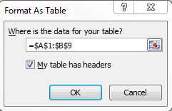
For a data table, you'll simply select a cell inside your data range, then go to the Home tab | Format as Table and select any of the available formats.

Excel will attempt to automatically determine your data range - assuming your data is laid out as in your example, with no empty rows or columns and headers at the top, it should be able to get the range automatically. If not, you can select it here.

Click OK, and your data table will be created.

A data table gives you a number of nifty features:

• The best one, for our purposes, is that it creates a named range, by default called Table1, that automatically expands if new data is added in the row directly below it or the column next to it.

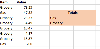
• The second best one, for our purposes is that you can used that named range in formulae. In your example, assuming the headers "Gas" and "Grocery" are in column D, we can put the following formula into column E: =SUMIF(Table1[Item],D4,Table1[Value]) This formula will look at the data table, Table1, and look at the Item column for all values that match the value in D4. Then it will sum the respective values from the Value column.

You can also use Table1 as the source for a PivotTable, but it won't automatically update as new data is added to the data table; you would need to go to the Pivot, right-click on it, and choose "Refresh".

Dynamic Named Range

To be clear, I recommend the Data Table option. It's cleaner, easier, and there's less room for things to go horribly wrong! However, if you prefer, we can look at a Dynamic Named Range. This would be necessary in older versions of Excel, and there are some situations where you might prefer it.

We're actually going to create two named ranges, using a very similar formula for each. In Excel 2007 and later, go to the Formulas tab and select Name Manager:

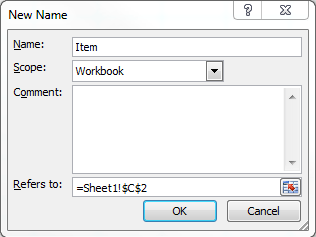
In the Name Manager Window click New to go to the New Name box. We're going to need two essential items here - a name, and Refers To formula. The name cannot have any spaces; in our case, we'll probably want to use Item:

In the Refers To box, we're going to put a formula. Note as you're typing this that the arrow keys will actually start selecting cells on the spreadsheet unless you hit F2 first. Enter the following: =OFFSET(Sheet1!$A$2,0,0,COUNTA(SHEET1!$A:$A)-1,1)

The OFFSET function used to return a range of cells, starting from a reference cell - in this case Sheet1!A2 - then moving down by a certain number of rows, and across by a certain number of columns. We're using 0,0 for that. It then returns a range that is a certain height and a certain width. We're using the COUNTA(A:A) to count how many cells in column A have values of any kind to get that height, then subtracting 1 to account for the fact that our data starts on row 2, and returning a range that is 1 column wide.

Create a second named range, the same as the first but with the name "Value" and the formula referring to column B: =OFFSET(Sheet1!$B$2,0,0,COUNTA(SHEET1!$B:$B)-1,1)

We can now use those named ranges as the sources for a similar formula to the one we used in the Data Table method: =SUMIF(Item,D4,Value)

You can also use dynamic named ranges to feed into a PivotTable, but in that case you'd want to change the ,1) to ,1), to return the entire data set.

Just use the entire column

All these methods are rather involved, but they avoid trying to use too many resources to accomplish the goal. If you're not worried about that, you can always use the simple option: Reference the entire column in your formulae.

Put a formula like this in your totals cells: =SUMIF($A:$A,D4,$B:$B) This includes all rows in columns A and B. It'll work, but with less panache than the other options.