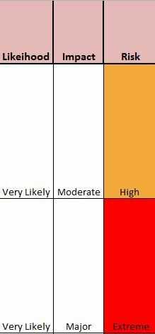
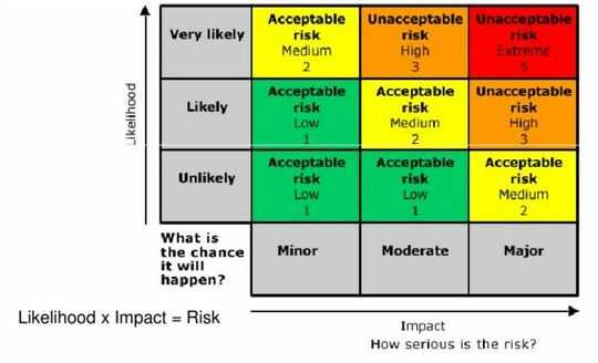
Personally, I'd create the risk chart as a table and then use index match pairs to find the row and column to locate the result you are seeking.
=index(RISK_TABLE_RANGE,MATCH(Likelihood_Cell,Likelihood_Range_RISKTABLE,0),
 MATCH(Risk_Cell,Impact_Range_RISKTABLE,0))
Essentially, you have the entire RISK_TABLE as one range and two additional ranges Likelihood_Range and Impact_Range which are the header/index for your risk table. You match on the two ranges and you get the cell coordinates for the RISK Level which appears in the square.
Think of it as a game of battleship where you ask "what row does very unlikely appear" and then "what column does major appear"


I put in the formula you posted and linked it to my risk table, but it did not place in Risk type after I filled in the Likelihood and Impact columns. Not sure why? – Morgan – 2016-12-19T22:24:50.317
You need to define three different named ranges: – berlin – 2016-12-19T22:58:17.497
You need to define three different named ranges:
Oh wow, I'm not sure how to do that. – Morgan – 2016-12-19T23:06:06.413
Go into Formulas -> Define Name – berlin – 2016-12-19T23:08:59.817
Go into Formulas -> Define Name
In my example the named ranges are called RISK_TABLE Likelihood_Range and Impact_Range
You can define the areas that they cover and then it should work. – berlin – 2016-12-19T23:10:02.820
Thank you. I got it to go through but it still doesn't do the function I'm looking for. The Risk field doesn't automatically fill in with a word, even after I put the Likelihood and Impact in. – Morgan – 2016-12-19T23:22:31.193
1Take the formula apart and see what you get for the two different parts. – berlin – 2016-12-20T15:29:58.553