Excel Pivot Table select rows based on column, with all columns displayed

I am using Excel 2010. Below is an anonymized sample of my data.

Name    Factor  Nick Town
Anton   0   Anton   Denver
Anton   1   Anton1  Boston
Anton   2   AntonB  Miami
Anton   1   Anton1  Seattle
Bernard 0   Bernard Denver
Bernard 1   Bernie  Miami
Bernard 1   Bernardo    Seattle
Chuck   0   Chuck   Denver
Chuck   1   Chuckee Chicago
Chuck   2   Chuckee Seattle
Chuck   2   Chucky  Miami
Chuck   1   Tchuk   Chicago
Chuck   2   Chuck   Houston
Deborah 0   Deborah Denver
Deborah 1   Deb Miami
Deborah 2   Debbie  Chicago
Deborah 3   Debbee  Boston
Deborah 1   Debbie  Boston

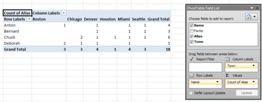
What I want: For each Name which is referred in a specific town (say Chicago), I want all the towns where they are referred.

Something like:

In SQL, I would have expressed that as:

select distinct Name , town from Dist 
  where Name in (select Name from Dist where town='Chicago');

My process: I need the list of towns for each Name. It is quite simple.

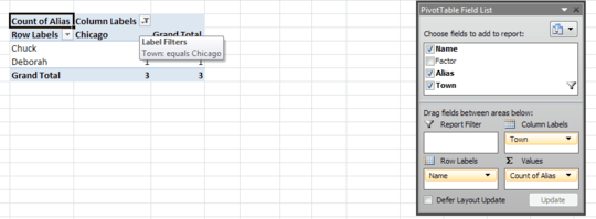
My issue comes in when I want this list filtered to only the Names having Chicago in their list. If I filter on Chicago, I get the following:

I tried to duplicate the town field to be able to filter on the first and display the second. This did not work.
I tried various moves between columns and rows, with no success.
I don't even see how to compute a column to reach my goal.

If this could be achieved without Pivot Tables, I am ok with this. I just thought it would be easier.

Mat M

Posted 2016-12-01T16:37:39.807

Reputation: 119

What's wrong with the result you achieved? Can you mock up what you want the result to look like? – OldUgly – 2016-12-04T20:48:11.160

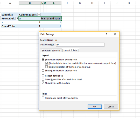
@OldUgly The result I want is the picture in "What I want". It is a mockup. The two last pictures are the one I can get; they are real screenshots. – Mat M – 2016-12-05T08:31:45.777

Well, actually, in the mockup, the Boston column should not be there. It is a leftover. – Mat M – 2016-12-09T13:19:20.697

Answers

You need to add a helper column to your source data. Supposing that name is in column A and Town is in column D, your formula will be (in E2):

=COUNTIF(A:A,A2,D:D,"Chicago")

This will return 1 for names having Chicago, and 0 for names without Chicago. (same logic as your subquery would do in SQL)

Just add this new column for your pivot table filter and filter for 1.

Máté Juhász

Posted 2016-12-01T16:37:39.807

Reputation: 16 807

It validates my second thought that I need one column for each town. Or, at least an external cell with the town I want to use as a filter. – Mat M – 2016-12-19T13:47:32.623

Select the column headers and right click. Select field settings > layout and print. And toggle show items with no data.

Serhat Cevikel

Posted 2016-12-01T16:37:39.807

Reputation: 219

This will display all cities, but won't display counts in them:( – Máté Juhász – 2016-12-15T20:24:37.437

Well, that's simply. If you want it to give the counts, then you should change the pivot table options so that, value field displays "count"? – Serhat Cevikel – 2016-12-15T20:36:22.160

This does not work. Try with the provided data sample. – Mat M – 2016-12-19T13:45:38.140