Determine United Airlines status level using worksheet functions

United Airlines MileagePlus Premier status levels are determined by a combination of criteria:

Silver: (PQM>=25000 OR PQS>=30) AND PQD>=3000
Gold: (PQM>=50000 OR PQS>=60) AND PQD>=6000
Platinum:(PQM>=75000 OR PQS>=90) AND PQD>=9000
1K: (PQM>=100000 OR PQS>=120) AND PQD>=12000

I have columns with the PQM, PQS and PQD totals. I'd like a formula to display the status level (e.g. "Gold"). Do I need a complex set of nested IF statements? Do I do a lookup somehow?

Drew McManus

Posted 2016-11-25T18:00:52.550

Reputation: 53

2You've specified several different spreadsheet applications. Is there any preference? – bwDraco – 2016-11-25T18:58:05.457

I would do (and just did) the nested IFs myself, would be interested to know if there's a better way too. I'm assuming you don't need answers showing how to structure that nested IF solution? – 3N1GM4 – 2016-11-25T20:23:36.300

@bwDraco I am using Numbers on MacOS. Function for that would be ideal, but I could adapt one if you are more confortable with Excel or Google Sheets. – Drew McManus – 2016-11-26T02:29:36.937

@3N1GM4 I have been fiddling with the nested IFs, but getting a lot of errors. If you have it working, I'd really appreciate a look. Thanks! – Drew McManus – 2016-11-26T02:30:55.853

Answers

Here is another approach using INDEX and MATCH, it's a more abstract, but also shorter formula based on your logic:

=INDEX(Table1[LEVEL],MIN(MAX(MATCH(B9,Table1[PQM]),MATCH(C9,Table1[PQS])),MATCH(D9,Table1[PQD])))

(PQM>=25000 OR PQS>=30) AND PQD>=3000

PQM>=25000 OR PQS>=30 - the higher level reached by PQM or PQS => MAX
(...) AND PQD>=3000 - the lower level reached by previous selection and PQD

Or just the formula without helper table:

=INDEX({"--","Silver","Gold","Platinum","1k"},MIN(MAX(MATCH(B9,{0,25000,50000,75000,100000}),MATCH(C9,{0,30,60,90,120})),MATCH(D9,{0,3000,6000,9000,12000})))

Máté Juhász

Posted 2016-11-25T18:00:52.550

Reputation: 16 807

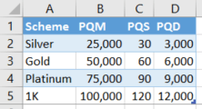
So if you did want to go with the nested IF solution, you could create a small lookup table like this:

And then if you have your PQM, PQS and PQD values in B8, C8 and D8 respectively, the formula would be:

=IF(AND(OR(B8>$B$5,C8>$C$5),D8>$D$5),$A$5,IF(AND(OR(B8>$B$4,C8>$C$4),D8>$D$4),$A$4,IF(AND(OR(B8>$B$3,C8>$C$3),D8>$D$3),$A$3,IF(AND(OR(B8>$B$2,C8>$C$2),D8>$D$2),$A$2,"None"))))

You could just as easily replace the table references with hard coded values if you'd rather not have the lookup table (although I prefer having it in case you need to change the parameters of the calculation in the future):

=IF(AND(OR(B8>100000,C8>120),D8>12000),"1K",IF(AND(OR(B8>75000,C8>90),D8>9000),"Platinum",IF(AND(OR(B8>50000,C8>60),D8>6000),"Gold",IF(AND(OR(B8>25000,C8>30),D8>3000),"Silver","None"))))

Hopefully it's fairly obvious how this works, it's checking for the highest level conditions first, then if they're not satisfied, working its way down the levels until it finds one which is, returning "None" if there is no applicable level to return.

3N1GM4

Posted 2016-11-25T18:00:52.550

Reputation: 398