How do I count rows with similar data in 2 columns as 1 data entry?

1

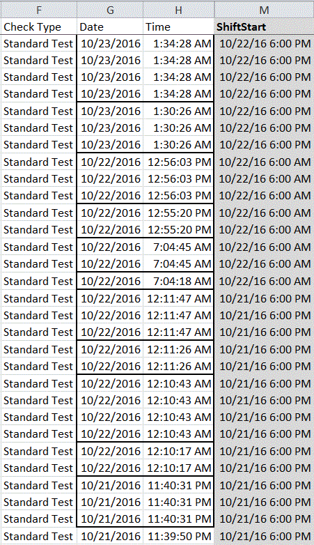
The SPC program test data is entered into is not able to perform compliance validation. Below is an image of data exported to excel. If the date and time are an exact match, it is considered 1 completed test. The number of rows will very based on columns not shown (Data that is collected). I have included a box around those rows that should be counted as 1 completed test.

I would like to be able to use a pivot table that will show the number of tests completed (not the number of rows) per shift start so that I can create trend charts to show compliance (Compliance requirements are in a calculated field). I am looking for suggestions on the best way to accomplish this (i.e. Helper column with a formula, pivot calculated field, etc.) so that I can quickly export/ import the data weekly and send out charts to my team.
enter image description here

Crainiac

Posted 2016-10-25T14:06:34.027

Reputation: 93

I've had this exact problem. I've heard that counting unique rows in a pivottable is a native feature of excel 2013, but I'll post my solution since you and I are both on 2010. – Some_Guy – 2016-10-25T14:25:31.427

Answers

1

I would add another column (N in your example) that would flag the last row of a complete test. Let's call this column "Unique Test". The formula would be:

=IF(OR(G2<>G3, H2<>H3), TRUE, FALSE)

Now, if you filter column N to show only TRUE values, you get a list of completed tests, one row per test.

Regardless of this filter, you can create a Pivot table to count tests per shift like this:

  1. Select columns M and N.
  2. Insert a PivotTable (on the Insert tab).
  3. Drag the ShiftStart field to the Row Labels area.
  4. Drag the Unique Test field to the Values area (getting Count of Unique Test as the value).
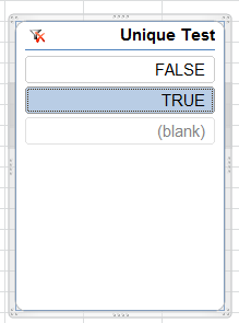
  5. On the PivotTable Tools, under the Options tab, click Insert Slicer, choose Unique Testand then click TRUE on the slicer.

    enter image description here

    enter image description here

Atzmon

Posted 2016-10-25T14:06:34.027

Reputation: 2 639

0

As mentioned above, pivot tables include this functionality in 2013 and later.


results

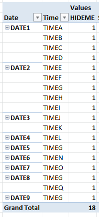
enter image description here enter image description here

Method

Assuming your data starts in row 2, The most calculation efficient and easier to understand way would seem to be:

=IF(COUNTIFS($G$2:G2,G2,$H$2:H2,H2)>1,0,1)

for x=2 to n, count the number of times Gx=Gn AND Hx=Hn

The countifs part counts the number of unique occurrences of both G&H up to that pount. With the IF, this will return 0 for repeated values and 1 for the very first occurrence of that combination of g and h.

Drag this to the bottom of your table, and add a sum of this column to your final pivot table, and you'll have a count of unique times and dates.

This works for non-contiguous data too, where repeated values are not consecutive (although it appears this wouldn't apply to your data).

for versions of excel which don't include =countifs:

SUMPRODUCT(($G$2:$G3=G3)*($H$3:$H3=H3))

Notice the $s. This formula will apply from row 2 until the current row, expanding the selection as it goes down. This sums the product TRUE and TRUE (1 and 1) for every row x from x=2 to x=n where both Gx=Gn and Hx=Hn. The current row (row n) is counted. If the combination is found earlier than the current row, the formula will count it (via the the sum of TRUE*TRUE).

In short, it counts the number of unique occurrences of both G and H. So PUT

N2=IF(SUMPRODUCT(($G$2:$G2=G2)*($H$2:$H2=H2))>1,0,1)


Some_Guy

Posted 2016-10-25T14:06:34.027

Reputation: 684

thank you for your solution. Neither of those solutions worked well with 'drag and copy' so I marked the other one as a solution. I will try to keep the suggestions you made in mind for other workbooks. – Crainiac – 2016-10-25T17:39:32.647

Hi crainiac, just trying to work out what do you mean here by drag and copy? Maybe I've made a mistake in my post, you should be able to just autofill the formula down to the bottom of the table. – Some_Guy – 2016-10-27T09:59:33.347

@Crainiac forgot to tag you – Some_Guy – 2016-10-27T15:28:46.167