How to select the first number in cell in Excel?

Question

I have a table that stores both a number and some text in a cell, and I want to do an arithmetic operation based on the numbers. So my table looks like this:

Number1       | Number2       | Product
2             | 3             | 6
3 (some text) | 40            | 120
4             | 5 (here too)  | 20

So in the presence of those ugly texts, I still want to be able to produce column 3 automatically. I guess I need a function that parses the substring upto the first non-numeric character into a number. Can I do this with Excel?

P.S.: The numbers can have more than 1 digits. Safe to assume they are integers, but it would be nice to see a solution that applies to floating points too :)

Thanks,

Answer 1

To get the numbers if they are in the beginning of the string we can use this:

=MID(A2,1,AGGREGATE(14,6,SEARCH("}}}",SUBSTITUTE(A2,{1,2,3,4,5,6,7,8,9,0},"}}}",LEN(A2)-LEN(SUBSTITUTE(A2,{1,2,3,4,5,6,7,8,9,0},"")))),1))

as our base formula, This will find the end of the number and return that as the end of the MID() Function.

There is a lot going on here:

SUBSTITUTE(A2,{1,2,3,4,5,6,7,8,9,0},"}}}",LEN(A2)-LEN(SUBSTITUTE(A2,{1,2,3,4,5,6,7,8,9,0},""))) As this part iterates through the numbers it is replacing the last instance of each number with }}}.

The third criterion of SUBSTITUTE is the instance. We find the number of instances with the LEN(A2)-LEN(SUBSTITUTE(A2,{1,2,3,4,5,6,7,8,9,0},"")). It iterates through the numbers and replaces each one at a time with nothing. It then finds the difference in length of the original string and the new one.

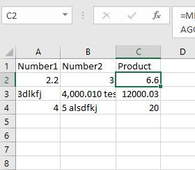
So in the case of A2 when it iterates to the 2 it finds 2 and the outer Substitute replaces the last one with }}}. This is just a temprorary place holder.

The Aggregate function is a multi function function. The 14 tells the funtions we are using the Large() function. The 6 tells the function to ignore errors. This is important in that many of the iteration will not find anything and return an error.

With the 1 at the end it tells the function we want the highest return from the Search function which searches for those temporary }}} that are placed through iteration on the last instance of each number.

So the Aggregate returns the max number found. Which we pass to the length criterion in the Mid function.

So we now have found the number at the front of the string.

So we can multiply two of these together to get the desired output(Any math function will turn the returned string into a number):

=MID(A2,1,AGGREGATE(14,6,SEARCH("}}}",SUBSTITUTE(A2,{1,2,3,4,5,6,7,8,9,0},"}}}",LEN(A2)-LEN(SUBSTITUTE(A2,{1,2,3,4,5,6,7,8,9,0},"")))),1))*MID(B2,1,AGGREGATE(14,6,SEARCH("}}}",SUBSTITUTE(B2,{1,2,3,4,5,6,7,8,9,0},"}}}",LEN(B2)-LEN(SUBSTITUTE(B2,{1,2,3,4,5,6,7,8,9,0},"")))),1))

One Caveat The Aggregate function was introduced in Excel 2010. It may not work with older versions.

If you have an older version you will need to use this longer formula:

=MID(A2,1,MAX(IF(ISNUMBER(SEARCH("}}}",SUBSTITUTE(A2,{1,2,3,4,5,6,7,8,9,0},"}}}",LEN(A2)-LEN(SUBSTITUTE(A2,{1,2,3,4,5,6,7,8,9,0},""))))),SEARCH("}}}",SUBSTITUTE(A2,{1,2,3,4,5,6,7,8,9,0},"}}}",LEN(A2)-LEN(SUBSTITUTE(A2,{1,2,3,4,5,6,7,8,9,0},"")))))))*MID(B2,1,MAX(IF(ISNUMBER(SEARCH("}}}",SUBSTITUTE(B2,{1,2,3,4,5,6,7,8,9,0},"}}}",LEN(B2)-LEN(SUBSTITUTE(B2,{1,2,3,4,5,6,7,8,9,0},""))))),SEARCH("}}}",SUBSTITUTE(B2,{1,2,3,4,5,6,7,8,9,0},"}}}",LEN(B2)-LEN(SUBSTITUTE(B2,{1,2,3,4,5,6,7,8,9,0},"")))))))

It does roughly the same as the one above accept it must test for the errors first before finding the max.

Answer 2

Assuming the number is always separated from any text by a space, you could use something like this. Say your example has data starting in A2, so your first result in C2 would ordinarily look like:

=A2*B2

We need to replace the simple cell references with a formula that treats the source cell as a number if it's only a number, but extracts the number if there's also text. So C2 would become:

=IF(ISNUMBER(A2),A2,LEFT(A2,FIND(" ",A2)-1)) * IF(ISNUMBER(B2),B2,LEFT(B2,FIND(" ",B2)-1))

If the source cell isn't a number, it finds the first space and returns the characters before it. Technically, what it returns is a text value containing digits, but Excel is smart enough to treat it as a number in calculating the product (no need to nest that inside another function to convert it to a number). And note that if the number is floating point, this will still work.

Caveat: This relies on "clean" source data, i.e., either a numeric entry, or a text entry where it starts with a number which is followed by a space. If there is a cell that doesn't conform to that, you would need to either clean up the data or include some form of error checking. The best solution would be to split the two data columns so that any text is in a separate cell.