Is there a dynamic sorting feature in Excel 2007/2010?

Question

I have a task list spreadsheet that I maintain. Each task is given a ranking based on number of days until due date, weighted by high, low, or medium priority. The ranking is automatically calculated, and the resulting list manually sorted to yield the current list of to-do's in priority order.

In a perfect world, I'd like to set up a second tab in my worksheet that would display the data from my first tab, but sort it for me on the fly. For instance, if I entered a new task that was due today with a high priority, I could flip to sheet 2 and it would already be automagically sorted to the top of the list.

Sheet One (as entered; number is calculated weight)

Task 01, 06/20/2013, Low,  0009
Task 02, 06/20/2013, High, 0999
Task 03, 06/30/2013, Med,  0089
Task 04, 06/19/2013, High, 1000  <-- new entry

Sheet Two (automatically sorted, descending order on calculated weight)

Task 04, 06/19/2013, High, 1000 
Task 02, 06/20/2013, High, 0999
Task 03, 06/30/2013, Med,  0089
Task 01, 06/20/2013, Low,  0009

We're transitioning from 2007 to 2010 in our organization, so I want to make sure that any soutions work in both versions. Any ideas?

Answer 1

Excel does this sort of thing easily. You shouldn't even need a second sheet (although you could certainly use one).

1. Convert your list of tasks to a Table Insert>Tables>Table.
2. In your Calculated Weight Column, use the drop down arrow and select Sort Largest to Smallest.
3. Each time you add a row to your table, just re-sort and you'll always have the highest priority first.

Here's what the Table and associated Pivot would look like. You could place them on the same or separate sheets, to your preference.

As an alternative, you could have this table feed a Pivot Table which would always be sorted in the same manner, but you'll still have to refresh the Pivot Table whenever you update the original data Table (whether manually or automatically based upon a time period or workbook open). This functionality is available in both 2007 and 2010.

Answer 2

This is how you sort data dynamically. The first one shows the results while the second one shows the equation used. Don't worry about the "C" Column being a bunch of random numbers. That's just the date converter that you don't have to understand. It's like computer formula for the date or something. Anyways the VLookups are all pretty much the same so it's easy. Rank column needs to be the far most left column. Since you put 0009 and all those other crazy numbers, I had to write them in as text rather than numbers. Because of this, I couldn't use rank to order them. So I created column "F" to convert the text 0009 to just 9 in number format. I used the Value function to do that. That pretty much covers it. Now you can hide columns A, F, and G if you don't want to see them. Just hold down the control button and select the entire columns of A, F, and G by clicking on the actual letters A, F, and G on the column labels. Then just right click one of those columns and find where it says hide.

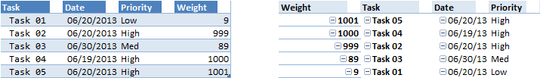
Sorry, I wanted to post a screen shot image of this but this website doesn't allow new users to post images. Here is the output table. I skipped the other columns because they would take up too much space on this website and they are almost exactly the same as columns G and H, so it shouldn't be that hard for you to figure it out.

   A|       B|         C|    D|      E|     F|       G|       H|         I|
Rank|   Tasks|      Date|  H-L| w-text| w-num| FinRank| VLookup|   VLookup|
   4| Task 01| 6/19/2013|  Low|   0009|     9|       1| Task 04| 6/19/2013|
   2| Task 02| 6/20/2013| High|   0999|   999|       2| Task 02| 6/20/2013|
   3| Task 03| 6/30/2013|  Med|   0089|    89|       3| Task 03| 6/30/2013|
   1| Task 04| 6/19/2013| High|   1000|  1000|       4| Task 01| 6/19/2013|

Here is the formulas

Column A, where it says 4: =RANK(F2,$F$2:$F$5,0)
Column A, where it says 2: =RANK(F3,$F$2:$F$5,0) and so on and so forth...
Columns B, C, D, and E are just text you input.
Column F, where the 9 is: =VALUE(E2)
Column F, where the 999 is: =VALUE(E3) and so on and so forth
Column G, is just numbers from 1 to whatever number you want. You just type them in. You need this to do the VLookup.
Column H, first row: =VLOOKUP(G2,$A$2:$F$5,2,FALSE)
Column H, second row: =VLOOKUP(G3,$A$2:$F$5,2,FALSE) and so on and so forth...

The rest of the columns are just like column H.
Column I row 1 looks like this: =VLOOKUP(G2,$A$2:$F$5,3,FALSE)
Column J row 1 looks like this: =VLOOKUP(G2,$A$2:$F$5,4,FALSE)
Column K row 1 looks like this: =VLOOKUP(G2,$A$2:$F$5,5,FALSE)
*See how there is only 1 difference between them? Easy right?