You can avoid the autofill feature completely with array formulas. Just enter the formula like normal but append :column at the end of each cell reference and then press Ctrl+Shift+Enter. The formula will then be applied immediately to all cells in the column without dragging anything
Edit:
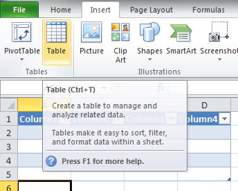
Newer Excel versions will automatically use array formulas to fill down when there's a new data row
Beginning with the September 2018 update for Office 365, any formula that can return multiple results will automatically spill them either down, or across into neighboring cells. This change in behavior is also accompanied by several new dynamic array functions. Dynamic array formulas, whether they’re using existing functions or the dynamic array functions, only need to be input into a single cell, then confirmed by pressing Enter. Earlier, legacy array formulas require first selecting the entire output range, then confirming the formula with Ctrl+Shift+Enter. They’re commonly referred to as CSE formulas.
Guidelines and examples of array formulas
If you're on an older version of Excel or want to know more about array formulas then continue reading
For example putting =B3:B + 2*C3:C in D3 and Ctrl+Shift+Enter is equivalent to typing =B3 + 2*C3 and dragging all the way down in a table starting from row 3
That's fast to type, but has a disadvantage that unused cells at the end (outside the current table) are still calculated and show 0. There's an easy way to hide the 0s. However the even better way is to limit the calculation to the last column of the table. Knowing that in an array formula you can use X3:X101 to apply to only cells from X3 to X101 we can use INDIRECT function to achieve the same effect
- Enter
=LOOKUP(2, 1/(A:A <> ""), A:A) in some cell outside the table to find the last non-blank cell in the table and name it LastRow. Alternatively use =COUNTA(A3:A) + 2 when the table's first row is 3
- Then instead of
B3:B use =INDIRECT("B3:B" & LastRow)
For example if you want cells in column D to contain the products of cells in B and C, and column E contains sums of B and C, instead of using D3 = B3*C3 and E3 = B3 + C3 and drag down you just put the below formulas in D3 and E3 respectively and press Ctrl+Shift+Enter
=INDIRECT("B3:B" & LastRow) * INDIRECT("C3:C" & LastRow)
=INDIRECT("B3:B" & LastRow) + INDIRECT("C3:C" & LastRow)
From now on every time you add data to a new row, the table will be automatically updated
Array formula is very fast since the data access pattern is already known. Now instead of doing 100001 different calculations separately, they can be vectorized and done in parallel, utilizing multiple cores and SIMD unit in the CPU. It also has the below advantages:
- Consistency: If you click any of the cells from E2 downward, you see the same formula. That consistency can help ensure greater accuracy.
- Safety: You cannot overwrite a component of a multi-cell array formula. For example, click cell E3 and press Delete. You have to either select the entire range of cells (E2 through E11) and change the formula for the entire array, or leave the array as is. As an added safety measure, you have to press Ctrl+Shift+Enter to confirm the change to the formula.
- Smaller file sizes: You can often use a single array formula instead of several intermediate formulas. For example, the workbook uses one array formula to calculate the results in column E. If you had used standard formulas (such as
=C2*D2, C3*D3, C4*D4…), you would have used 11 different formulas to calculate the same results.
Guidelines and examples of array formulas
For more information read

They must be at least four. – Luke – 2018-05-07T07:39:00.673
@PeterL.,, nice interpretation +10 ☺ – Rajesh S – 2019-09-14T04:24:42.257
Interestingly, I can only get this to work in columns, not rows (e.g. if you transpose your example, I cannot get it to work). – RipperDoc – 2013-02-22T00:51:13.680
I have no idea why so... Perhaps because data usually stored in column mode with growing down - it's like more natural)) – Peter L. – 2013-02-22T05:50:57.997