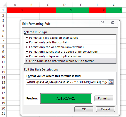
1
I have a row containing, let's say, the following values:
0, empty, empty, 1, empty, 0, 1
I want to apply a conditional formatting so that:
- cell 0: background is RED
- cell 1: background is GREEN
- cell empty: background is equal to the previous cell background
the result should be:
RED, RED, RED, GREEN, GREEN, RED, GREEN
The question is: using conditional formatting, how to apply to a cell the format of a previous cell ?
thank you in advance for any comment

Thank you Máté, the solution effectively solves the question posted. Moreover your approach 'evaluate true if 1 or empty' is interesting and I'm wondering if it is possible to apply it to a real case, in which I have a pivottable with 'expandable' cells – Roberto Vanoli – 2016-09-05T13:27:48.140
I don't really understand your example with the pivottable. Maybe you can ask it a new question and add some sample data. – Máté Juhász – 2016-09-05T13:35:42.030
I've solved my problem using pivotable and your formula, and I prepared a detailed post of the solution. Unfortunately I cannot publish it because it contain images and I have not enought reputation for that (I need 10 I have 3). If you think my question is interesting, please upvote this post so that I earn the missing points and can publish the solution. thank you RV – Roberto Vanoli – 2016-09-06T07:45:09.860
@RobertoVanoli you can still post your solution, please upload your pictures to imgur and include their link in your answer, somebody with enough reputation will include them for you. – Máté Juhász – 2016-09-06T07:48:17.613
I have posted a sample of using your formula with a pivotable here http://superuser.com/questions/1121432/how-to-apply-conditional-formatting-of-an-adiacent-row-in-a-pivotable-when-the-c
– Roberto Vanoli – 2016-09-06T08:41:06.193