Mathieu function
In mathematics, Mathieu functions, sometimes called angular Mathieu functions, are solutions of Mathieu's differential equation

where and are parameters. They were first introduced by Émile Léonard Mathieu, who encountered them while studying vibrating elliptical drumheads.[1][2] They have applications in many fields of the physical sciences, such as optics, quantum mechanics, and general relativity. They tend to occur in problems involving periodic motion, or in the analysis of partial differential equation boundary value problems possessing elliptic symmetry.[3]


Definition
Mathieu functions
In some usages, Mathieu function refers to solutions of the Mathieu differential equation for arbitrary values of and . When no confusion can arise, other authors use the term to refer specifically to - or -periodic solutions, which exist only for special values of and .[4] More precisely, for given (real) such periodic solutions exist for an infinite number of values of , called characteristic numbers, conventionally indexed as two separate sequences and , for . The corresponding functions are denoted and , respectively. They are sometimes also referred to as cosine-elliptic and sine-elliptic, or Mathieu functions of the first kind.


As a result of assuming that is real, both the characteristic numbers and associated functions are real-valued.[5]
and can be further classified by parity and periodicity (both with respect to ), as follows:[4]

Function Parity Period even even odd odd


The indexing with the integer , besides serving to arrange the characteristic numbers in ascending order, is convenient in that and become proportional to and as . With being an integer, this gives rise to the classification of and as Mathieu functions (of the first kind) of integral order. For general and , solutions besides these can be defined, including Mathieu functions of fractional order as well as non-periodic solutions.


Modified Mathieu functions
Closely related are the modified Mathieu functions, also known as radial Mathieu functions, which are solutions of Mathieu's modified differential equation

which can be related to the original Mathieu equation by taking . Accordingly, the modified Mathieu functions of the first kind of integral order, denoted by and , are defined from[6]


These functions are real-valued when is real.
Normalization
A common normalization,[7] which will be adopted throughout this article, is to demand

as well as require and as .


Floquet theory
Many properties of the Mathieu differential equation can be deduced from the general theory of ordinary differential equations with periodic coefficients, called Floquet theory. The central result is Floquet's theorem:


It is natural to associate the characteristic numbers with those values of which result in .[9] Note, however, that the theorem only guarantees the existence of at least one solution satisfying , when Mathieu's equation in fact has two independent solutions for any given , . Indeed, it turns out that with equal to one of the characteristic numbers, Mathieu's equation has only one periodic solution (that is, with period or ), and this solution is one of the , . The other solution is nonperiodic, denoted and , respectively, and referred to as a Mathieu function of the second kind.[10] This result can be formally stated as Ince's theorem:


An equivalent statement of Floquet's theorem is that Mathieu's equation admits a complex-valued solution of form

where is a complex number, the Floquet exponent (or sometimes Mathieu exponent), and is a complex valued function periodic in with period . An example is plotted to the right.


Other types of Mathieu functions
Second kind
Since Mathieu's equation is a second order differential equation, one can construct two linearly independent solutions. Floquet's theory says that if is equal to a characteristic number, one of these solutions can be taken to be periodic, and the other nonperiodic. The periodic solution is one of the and , called a Mathieu function of the first kind of integral order. The nonperiodic one is denoted either and , respectively, and is called a Mathieu function of the second kind (of integral order). The nonperiodic solutions are unstable, that is, they diverge as .[12]

The second solutions corresponding to the modified Mathieu functions and are naturally defined as and .


Fractional order
Mathieu functions of fractional order can be defined as those solutions and , a non-integer, which turn into and as .[6] If is irrational, they are non-periodic; however, they remain bounded as .


An important property of the solutions and , for non-integer, is that they exist for the same value of . In contrast, when is an integer, and never occur for the same value of . (See Ince's Theorem above.)
These classifications are summarized in the table below. The modified Mathieu function counterparts are defined similarly.
Classification of Mathieu functions[13] Order First kind Second kind Integral Integral Fractional ( non-integral)
Explicit representation and computation
First kind
Mathieu functions of the first kind can be represented as Fourier series:[4]

The expansion coefficients and are functions of but independent of . By substitution into the Mathieu equation, they can be shown to obey three-term recurrence relations in the lower index. For instance, for each one finds[14]


Being a second-order recurrence in the index , one can always find two independent solutions and such that the general solution can be expressed as a linear combination of the two: . Moreover, in this particular case, an asymptotic analysis[15] shows that one possible choice of fundamental solutions has the property


In particular, is finite whereas diverges. Writing , we therefore see that in order for the Fourier series representation of to converge, must be chosen such that . These choices of correspond to the characteristic numbers.

In general, however, the solution of a three-term recurrence with variable coefficients cannot be represented in a simple manner, and hence there is no simple way to determine from the condition . Moreover, even if the approximate value of a characteristic number is known, it cannot be used to obtain the coefficients by numerically iterating the recurrence towards increasing . The reason is that as long as only approximates a characteristic number, is not identically and the divergent solution eventually dominates for large enough .


To overcome these issues, more sophisticated semi-analytical/numerical approaches are required, for instance using a continued fraction expansion,[16][4] casting the recurrence as a matrix eigenvalue problem,[17] or implementing a backwards recurrence algorithm.[15] The complexity of the three-term recurrence relation is one of the reasons there are few simple formulas and identities involving Mathieu functions.[18]
In practice, Mathieu functions and the corresponding characteristic numbers can be calculated using pre-packaged software, such as Mathematica, Maple, MATLAB, and SciPy. For small values of and low order , they can also be expressed perturbatively as power series of , which can be useful in physical applications.[19]
Second kind
There are several ways to represent Mathieu functions of the second kind.[20] One representation is in terms of Bessel functions:[21]

where , and and are Bessel functions of the first and second kind.


Properties
There are relatively few analytic expressions and identities involving Mathieu functions. Moreover, unlike many other special functions, the solutions of Mathieu's equation cannot in general be expressed in terms of hypergeometric functions. This can be seen by transformation of Mathieu's equation to algebraic form, using the change of variable :


Since this equation has an irregular singular point at infinity, it cannot be transformed into an equation of the hypergeometric type.[18]
Qualitative behavior
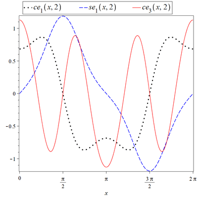
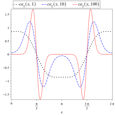

For small , and behave similarly to and . For arbitrary , they may deviate significantly from their trigonometric counterparts; however, they remain periodic in general. Moreover, for any real , and have exactly simple zeros in , and as the zeros cluster about .[25][26]


For and as the modified Mathieu functions tend to behave as damped periodic functions.

In the following, the and factors from the Fourier expansions for and may be referenced (see Explicit representation and computation). They depend on and but are independent of .


Reflections and translations
Due to their parity and periodicity, and have simple properties under reflections and translations by multiples of :[6]

One can also write functions with negative in terms of those with positive :[4][27]

Moreover,

Orthogonality and completeness
Like their trigonometric counterparts and , the periodic Mathieu functions and satisfy orthogonality relations

Moreover, with fixed and treated as the eigenvalue, the Mathieu equation is of Sturm-Liouville form. This implies that the eigenfunctions and form a complete set, i.e. any - or -periodic function of can be expanded as a series in and .[3]
Integral identities
Solutions of Mathieu's equation satisfy a class of integral identities with respect to kernels that are solutions of


More precisely, if solves Mathieu's equation with given and , then the integral


where is a path in the complex plane, also solves Mathieu's equation with the same and , provided the following conditions are met:[28]

- solves
- In the regions under consideration, exists and is analytic
- has the same value at the endpoints of


Using an appropriate change of variables, the equation for can be transformed into the wave equation and solved. For instance, one solution is . Examples of identities obtained in this way are[29]


Identities of the latter type are useful for studying asymptotic properties of the modified Mathieu functions.[30]
There also exist integral relations between functions of the first and second kind, for instance:[21]

valid for any complex and real .
Asymptotic expansions
The following asymptotic expansions hold for , , , and :[31]


Thus, the modified Mathieu functions decay exponentially for large real argument. Similar asymptotic expansions can be written down for and ; these also decay exponentially for large real argument.


One can also derive asymptotic expansions for large .[32] For the characteristic numbers in particular, one has

In the second reference, terms of this expansion are obtained explicitly up to and including the term of order . In addition, the splitting of the characteristic numbers (in quantum mechanics called eigenvalues) corresponding to even and odd periodic Mathieu functions is calculated from their boundary conditions. In quantum mechanics this provides the splitting of the eigenvalues into energy bands.

Applications
Mathieu's differential equations appear in a wide range of contexts in engineering, physics, and applied mathematics. Many of these applications fall into one of two general categories: 1) the analysis of partial differential equations in elliptic geometries, and 2) dynamical problems which involve forces that are periodic in either space or time. Examples within both categories are discussed below.
Partial differential equations
Mathieu functions arise when separation of variables in elliptic coordinates is applied to 1) the Laplace equation in 3 dimensions, and 2) the Helmholtz equation in either 2 or 3 dimensions. Since the Helmholtz equation is a prototypical equation for modeling the spatial variation of classical waves, Mathieu functions can be used to describe a variety of wave phenomena. For instance, in computational electromagnetics they can be used to analyze the scattering of electromagnetic waves off elliptic cylinders, and wave propagation in elliptic waveguides.[33] In general relativity, an exact plane wave solution to the Einstein field equation can be given in terms of Mathieu functions.
More recently, Mathieu functions have been used to solve a special case of the Smoluchowski equation, describing the steady-state statistics of self-propelled particles.[34]
The remainder of this section details the analysis for the two-dimensional Helmholtz equation.[35] In rectangular coordinates, the Helmholtz equation is

Elliptic coordinates are defined by

where , , and is a positive constant. The Helmholtz equation in these coordinates is


The constant curves are confocal ellipses with focal length ; hence, these coordinates are convenient for solving the Helmholtz equation on domains with elliptic boundaries. Separation of variables via yields the Mathieu equations


where is a separation constant.
As a specific physical example, the Helmholtz equation can be interpreted as describing normal modes of an elastic membrane under uniform tension. In this case, the following physical conditions are imposed:[36]
- Periodicity with respect to , i.e.
- Continuity of displacement across the interfocal line:
- Continuity of derivative across the interfocal line:


For given , this restricts the solutions to those of the form and , where . This is the same as restricting allowable values of , for given . Restrictions on then arise due to imposition of physical conditions on some bounding surface, such as an elliptic boundary defined by . For instance, clamping the membrane at imposes , which in turn requires


These conditions define the normal modes of the system.
Dynamical problems
In dynamical problems with periodically varying forces, the equation of motion sometimes takes the form of Mathieu's equation. In such cases, knowledge of the general properties of Mathieu's equation— particularly with regard to stability of the solutions—can be essential for understanding qualitative features of the physical dynamics.[37] A classic example along these lines is the inverted pendulum.[38] Other examples are
- vibrations of a string with periodically varying tension[37]
- stability of railroad rails as trains drive over them
- seasonally forced population dynamics
- the phenomenon of parametric resonance in forced oscillators
- motion of ions in a quadrupole ion trap[39]
- the Stark effect for a rotating electric dipole
- the Floquet theory of the stability of limit cycles
Quantum mechanics
Mathieu functions play a role in certain quantum mechanical systems, particularly those with spatially periodic potentials such as the quantum pendulum and crystalline lattices.
The modified Mathieu equation also arises when describing the quantum mechanics of singular potentials. For the particular singular potential the radial Schrödinger equation


can be converted into the equation

The transformation is achieved with the following substitutions

By solving the Schrödinger equation (for this particular potential) in terms of solutions of the modified Mathieu equation, scattering properties such as the S-matrix and the absorptivity can be obtained.[40]
See also
Notes
- Mathieu (1868).
- Morse and Feshbach (1953).
- Gutiérrez-Vega (2015).
- Arscott (1964), chapter III
- Arscott (1964) 43–44
- McLachlan (1947), chapter II.
- Arscott (1964); Iyanaga (1980); Gradshteyn (2007); This is also the normalization used by the computer algebra system Maple.
- Arscott (1964), p. 29.
- It is not true, in general, that a periodic function has the property . However, this turns out to be true for functions which are solutions of Mathieu's equation.
- McLachlan (1951), pp. 141-157, 372
- Arscott (1964), p. 34
- McLachlan (1947), p. 144
- McLachlan (1947), p. 372
- McLachlan (1947), p. 28
- Wimp (1984), pp. 83-84
- McLachlan (1947)
- Chaos-Cador and Ley-Koo (2001)
- Temme (2015), p. 234
- Müller-Kirsten (2012), pp. 420-428
- Meixner and Schäfke (1954); McLachlan (1947)
- Malits (2010)
- Jin and Zhang (1996)
- Van Buren and Boisvert (2007)
- Bibby and Peterson (2013)
- Meixner and Schäfke (1954), p.134
- McLachlan (1947), pp. 234–235
- Gradshteyn (2007), p. 953
- Arscott (1964), pp. 40-41
- Gradshteyn (2007), pp. 763–765
- Arscott (1964), p. 86
- McLachlan (1947), chapter XI
- McLachlan (1947), p. 237; Dingle and Müller-Kirsten (1962); Müller-Kirsten and Roquette (1962); Dingle and Müller-Kirsten (1964)
- Bibby and Peterson (2013); Barakat (1963); Sebak and Shafai (1991); Kretzschmar (1970)
- Solon et al (2015)
- see Willatzen and Voon (2011), pp. 61–65
- McLachlan (1947), pp. 294–297
- Meixner and Schäfke (1954), pp. 324–343
- Ruby (1996)
- March (1997)
- Müller-Kirsten (2006)

References
- Arscott, Felix (1964). Periodic differential equations: an introduction to Mathieu, Lamé, and allied functions. Pergamon Press. ISBN 9781483164885.
- Barakat, R. (1963), "Diffraction of Plane Waves by an Elliptic Cylinder", The Journal of the Acoustical Society of America, 35 (12): 1990–1996, Bibcode:1963ASAJ...35.1990B, doi:10.1121/1.1918878
- Bibby, Malcolm M.; Peterson, Andrew F. (2014). Accurate Computation of Mathieu Functions. Morgan & Claypool. doi:10.2200/S00526ED1V01Y201307CEM032. ISBN 9781627050852.
- Chaos-Cador, L.; Ley-Koo, E. (2002), "Mathieu functions revisited: matrix evaluation and generating functions", Revista mexicana de física, 48 (1): 67–75
- Dingle, R.B.; Müller, H.J.W. (1964). "The Form of the Coefficients of the Late Terms in Asymptotic Expansions of the Characteristic Numbers of Mathieu and Spheroidal-Wave Functions". Journal für die reine und angewandte Mathematik. 216: 123–133. ISSN 0075-4102.
- Gradshteyn, Izrail Solomonovich; et al. (February 2007). Jeffrey, Alan; Zwillinger, Daniel (eds.). Table of Integrals, Series, and Products. Translated by Scripta Technica, Inc. (7 ed.). Academic Press, Inc. ISBN 978-0-12-373637-6. MR 2360010.
- Gutiérrez-Vega, Julio C. (2015), "Mathieu Functions", in Nicholas J. Higham; et al. (eds.), The Princeton Companion to Applied Mathematics, Princeton University Press, pp. 159–160
- Iyanaga, Shōkichi; Kawada, Yukiyosi, eds. (1980) [1977]. Encyclopedic Dictionary of Mathematics, Volume I. Translated from the 2nd Japanese edition, paperback version of the 1977 edition (1st ed.). MIT Press. ISBN 978-0-262-59010-5. MR 0591028.
- Jin, J.M.; Zhang, Shan Jjie (1996). Computation of special functions. New York: Wiley. ISBN 9780471119630.
- Kretzschmar, J.G. (1970), "Wave Propagation in Hollow Conducting Elliptical Waveguides", IEEE Transactions on Microwave Theory and Techniques, 18 (9): 547–554, Bibcode:1970ITMTT..18..547K, doi:10.1109/TMTT.1970.1127288
- Malits, Pinchas (2010), "Relations between Mathieu functions of the first and second kind", Integral Transforms and Special Functions, 21 (6): 423–436, doi:10.1080/10652460903360499
- March, Raymond E. (April 1997). "An Introduction to Quadrupole Ion Trap Mass Spectrometry". Journal of Mass Spectrometry. 32 (4): 351–369. Bibcode:1997JMSp...32..351M. doi:10.1002/(SICI)1096-9888(199704)32:4<351::AID-JMS512>3.0.CO;2-Y.
- Mathieu, E. (1868), "Mémoire sur Le Mouvement Vibratoire d'une Membrane de forme Elliptique", Journal de Mathématiques Pures et Appliquées: 137–203
- McLachlan, N. W. (1951). Theory and application of Mathieu functions. Oxford University Press. Note: Reprinted lithographically in Great Britain at the University Press, Oxford, 1951 from corrected sheets of the (1947) first edition.
- Meixner, Josef; Schäfke, Friedrich Wilhelm (1954). Mathieusche Funktionen und Sphäroidfunktionen (in German). Berlin: Springer-Verlag. doi:10.1007/978-3-662-00941-3. ISBN 978-3-540-01806-3.
- Morse, Philip McCord; Feshbach, Herman (1953-01-01). Methods of Theoretical Physics: Pt. 1 (Reprint ed.). Boston, Mass: McGraw-Hill Inc.,US. ISBN 9780070433168.
- Müller-Kirsten, Harald J.W. (2006). Introduction to Quantum Mechanics: Schrödinger Equation and Path Integral. World Scientific. ISBN 981-256-692-9.
- Müller-Kirsten, H.J.W.; Dingle, R.B. (1962). "Asymptotic Expansions of Mathieu Functions and their Characteristic Numbers". Journal für die reine und angewandte Mathematik. 1962 (211): 11–32. doi:10.1515/crll.1962.211.11. ISSN 0075-4102.
- Müller-Kirsten, H.J.W. (1962). "On Asymptotic Expansions of Mathieu Functions". Journal für die reine und angewandte Mathematik. 1962 (211): 179–190. doi:10.1515/crll.1962.211.179. ISSN 0075-4102.
- Sebak, A.; Shafai, L. (1991), "Generalized solutions for electromagnetic scattering by elliptical structures", Computer Physics Communications, 68 (1–3): 315–330, Bibcode:1991CoPhC..68..315S, doi:10.1016/0010-4655(91)90206-Z
- Solon, A.P.; Cates, M.E.; Tailleur, J. (2015), "Active brownian particles and run-and-tumble particles: A comparative study", The European Physical Journal Special Topics, 224 (7): 1231–1262, arXiv:1504.07391, Bibcode:2015EPJST.224.1231S, doi:10.1140/epjst/e2015-02457-0
- Temme, Nico M. (2015), "Special Functions", in Nicholas J. Higham; et al. (eds.), The Princeton Companion to Applied Mathematics, Princeton University Press, p. 234
- Van Buren, Arnie L.; Boisvert, Jeffrey E. (2007). "Accurate calculation of the modified Mathieu functions of integer order". Quarterly of Applied Mathematics. 65 (1): 1–23. doi:10.1090/S0033-569X-07-01039-5. ISSN 0033-569X.
- Lew Yan Voon LC, Willatzen M (2011). Separable Boundary-Value Problems in Physics. Wiley-VCH. doi:10.1002/9783527634927. ISBN 978-3-527-41020-0. (free online access to the appendix on Mathieu functions)
- Wimp, Jet (1984). Computation with Recurrence Relations. Pitman Publishing. pp. 83–84. ISBN 0-273-08508-5.
- Wolf, G. (2010), "Mathieu Functions and Hill's Equation", in Olver, Frank W. J.; Lozier, Daniel M.; Boisvert, Ronald F.; Clark, Charles W. (eds.), NIST Handbook of Mathematical Functions, Cambridge University Press, ISBN 978-0-521-19225-5, MR 2723248
External links
- Weisstein, Eric W. "Mathieu function". MathWorld.
- List of equations and identities for Mathieu Functions functions.wolfram.com
- "Mathieu functions", Encyclopedia of Mathematics, EMS Press, 2001 [1994]
- Timothy Jones, Mathieu's Equations and the Ideal rf-Paul Trap (2006)
- Mathieu equation, EqWorld
- NIST Digital Library of Mathematical Functions: Mathieu Functions and Hill's Equation