History of Lorentz transformations

The history of Lorentz transformations comprises the development of linear transformations forming the Lorentz group or Poincaré group preserving the Lorentz interval ${\displaystyle -x_{0}^{2}+\cdots +x_{n}^{2}}$ and the Minkowski inner product ${\displaystyle -x_{0}y_{0}+\cdots +x_{n}y_{n}}$.

In mathematics, transformations equivalent to what was later known as Lorentz transformations in various dimensions were discussed in the 19th century in relation to the theory of quadratic forms, hyperbolic geometry, Möbius geometry, and sphere geometry, which is connected to the fact that the group of motions in hyperbolic space, the Möbius group or projective special linear group, and the Laguerre group are isomorphic to the Lorentz group.

In physics, Lorentz transformations became known at the beginning of the 20th century, when it was discovered that they exhibit the symmetry of Maxwell's equations. Subsequently, they became fundamental to all of physics, because they formed the basis of special relativity in which they exhibit the symmetry of Minkowski spacetime, making the speed of light invariant between different inertial frames. They relate the spacetime coordinates of two arbitrary inertial frames of reference with constant relative speed v. In one frame, the position of an event is given by x,y,z and time t, while in the other frame the same event has coordinates x′,y′,z′ and t′.

Overview

Most general Lorentz transformations

The general quadratic form q(x) with coefficients of a symmetric matrix A, the associated bilinear form b(x,y), and the linear transformations of q(x) and b(x,y) into q(x′) and b(x′,y′) using the transformation matrix g, can be written as[1]

${\displaystyle {\begin{matrix}{\begin{aligned}{\begin{aligned}q=\sum _{0}^{n}A_{ij}x_{i}x_{j}=\mathbf {x} ^{\mathrm {T} }\cdot \mathbf {A} \cdot \mathbf {x} \end{aligned}}&=q'=\mathbf {x} ^{\mathrm {\prime T} }\cdot \mathbf {A} '\cdot \mathbf {x} '\\b=\sum _{0}^{n}A_{ij}x_{i}y_{j}=\mathbf {x} ^{\mathrm {T} }\cdot \mathbf {A} \cdot \mathbf {y} &=b'=\mathbf {x} ^{\mathrm {\prime T} }\cdot \mathbf {A} '\cdot \mathbf {y} '\end{aligned}}\quad \left(A_{ij}=A_{ji}\right)\\\hline \left.{\begin{aligned}x_{i}^{\prime }&=\sum _{j=0}^{n}g_{ij}x_{j}=\mathbf {g} \cdot \mathbf {x} \\x_{i}&=\sum _{j=0}^{n}g_{ij}^{(-1)}x_{j}^{\prime }=\mathbf {g} ^{-1}\cdot \mathbf {x} '\end{aligned}}\right|\mathbf {g} ^{\rm {T}}\cdot \mathbf {A} \cdot \mathbf {g} =\mathbf {A} '\end{matrix}}}$

(Q1)

The case n=1 is the binary quadratic form introduced by Lagrange (1773) and Gauss (1798/1801), n=2 is the ternary quadratic form introduced by Gauss (1798/1801), n=3 is the quaternary quadratic form etc.

The general Lorentz transformation follows from (Q1) by setting A=A′=diag(-1,1,...,1) and det g=±1. It forms an indefinite orthogonal group called the Lorentz group O(1,n), while the case det g=+1 forms the restricted Lorentz group SO(1,n). The quadratic form q(x) becomes the Lorentz interval in terms of an indefinite quadratic form of Minkowski space (being a special case of pseudo-Euclidean space), and the associated bilinear form b(x) becomes the Minkowski inner product:[2][3]

${\displaystyle {\begin{matrix}{\begin{aligned}-x_{0}^{2}+\cdots +x_{n}^{2}&=-x_{0}^{\prime 2}+\dots +x_{n}^{\prime 2}\\-x_{0}y_{0}+\cdots +x_{n}y_{n}&=-x_{0}^{\prime }y_{0}^{\prime }+\cdots +x_{n}^{\prime }y_{n}^{\prime }\end{aligned}}\\\hline \left.{\begin{matrix}\mathbf {x} '=\mathbf {g} \cdot \mathbf {x} \\\downarrow \\{\begin{aligned}x_{0}^{\prime }&=x_{0}g_{00}+x_{1}g_{01}+\dots +x_{n}g_{0n}\\x_{1}^{\prime }&=x_{0}g_{10}+x_{1}g_{11}+\dots +x_{n}g_{1n}\\&\dots \\x_{n}^{\prime }&=x_{0}g_{n0}+x_{1}g_{n1}+\dots +x_{n}g_{nn}\end{aligned}}\\\\\mathbf {x} =\mathbf {g} ^{-1}\cdot \mathbf {x} '\\\downarrow \\{\begin{aligned}x_{0}&=x_{0}^{\prime }g_{00}-x_{1}^{\prime }g_{10}-\dots -x_{n}^{\prime }g_{n0}\\x_{1}&=-x_{0}^{\prime }g_{01}+x_{1}^{\prime }g_{11}+\dots +x_{n}^{\prime }g_{n1}\\&\dots \\x_{n}&=-x_{0}^{\prime }g_{0n}+x_{1}^{\prime }g_{1n}+\dots +x_{n}^{\prime }g_{nn}\end{aligned}}\end{matrix}}\right|{\begin{matrix}{\begin{aligned}\mathbf {A} \cdot \mathbf {g} ^{\mathrm {T} }\cdot \mathbf {A} &=\mathbf {g} ^{-1}\\\mathbf {g} ^{\rm {T}}\cdot \mathbf {A} \cdot \mathbf {g} &=\mathbf {A} \\\mathbf {g} \cdot \mathbf {A} \cdot \mathbf {g} ^{\mathrm {T} }&=\mathbf {A} \\\\\end{aligned}}\\{\begin{aligned}\sum _{i=1}^{n}g_{ij}g_{ik}-g_{0j}g_{0k}&=\left\{{\begin{aligned}-1\quad &(j=k=0)\\1\quad &(j=k>0)\\0\quad &(j\neq k)\end{aligned}}\right.\\\sum _{j=1}^{n}g_{ij}g_{kj}-g_{i0}g_{k0}&=\left\{{\begin{aligned}-1\quad &(i=k=0)\\1\quad &(i=k>0)\\0\quad &(i\neq k)\end{aligned}}\right.\end{aligned}}\end{matrix}}\end{matrix}}}$

(1a)

Such general Lorentz transformations (1a) for various dimensions were used by Gauss (1818), Jacobi (1827, 1833), Lebesgue (1837), Bour (1856), Somov (1863), Hill (1882) in order to simplify computations of elliptic functions and integrals.[4][5] They were also used by Poincaré (1881), Cox (1881/82), Picard (1882, 1884), Killing (1885, 1893), Gérard (1892), Hausdorff (1899), Woods (1901, 1903), Liebmann (1904/05) to describe hyperbolic motions (i.e. rigid motions in the hyperbolic plane or hyperbolic space), which were expressed in terms of Weierstrass coordinates of the hyperboloid model satisfying the relation ${\displaystyle -x_{0}^{2}+\cdots +x_{n}^{2}=-1}$ or in terms of the Cayley–Klein metric of projective geometry using the "absolute" form ${\displaystyle -x_{0}^{2}+\cdots +x_{n}^{2}=0}$.[M 1][6][7] In addition, infinitesimal transformations related to the Lie algebra of the group of hyperbolic motions were given in terms of Weierstrass coordinates ${\displaystyle -x_{0}^{2}+\cdots +x_{n}^{2}=-1}$ by Killing (1888-1897).

If ${\displaystyle x_{i},\ x_{i}^{\prime }}$ in (1a) are interpreted as homogeneous coordinates, then the corresponding inhomogenous coordinates ${\displaystyle u_{s},\ u_{s}^{\prime }}$ follow by

${\displaystyle \left[{\frac {x_{0}}{x_{0}}},\ {\frac {x_{s}}{x_{0}}}\right]=\left[1,\ u_{s}\right],\ \left[{\frac {x_{0}^{\prime }}{x_{0}^{\prime }}},\ {\frac {x_{s}^{\prime }}{x_{0}^{\prime }}}\right]=\left[1,\ u_{s}^{\prime }\right],\ (s=1,2\dots n)}$

so that the Lorentz transformation becomes a homography leaving invariant the equation of the unit sphere, which John Lighton Synge called "the most general formula for the composition of velocities" in terms of special relativity (the transformation matrix g stays the same as in (1a)):[8]

${\displaystyle {\begin{matrix}{\begin{matrix}-x_{0}^{2}+\cdots +x_{n}^{2}=-x_{0}^{\prime 2}+\dots +x_{n}^{\prime 2}&\rightarrow &{\begin{aligned}-1+u_{1}^{2}+\cdots +u_{n}^{2}&={\scriptstyle {\frac {-1+u_{1}^{\prime 2}+\cdots +u_{n}^{\prime 2}}{\left(g_{00}+g_{01}u_{1}^{\prime }+\dots +g_{0n}u_{n}^{\prime }\right)^{2}}}}\\{\scriptstyle {\frac {-1+u_{1}^{2}+\cdots +u_{n}^{2}}{\left(g_{00}-g_{10}u_{1}-\dots -g_{n0}u_{n}\right)^{2}}}}&=-1+u_{1}^{\prime 2}+\cdots +u_{n}^{\prime 2}\end{aligned}}\\\hline -x_{0}^{2}+\cdots +x_{n}^{2}=-x_{0}^{\prime 2}+\dots +x_{n}^{\prime 2}=0&\rightarrow &-1+u_{1}^{2}+\cdots +u_{n}^{2}=-1+u_{1}^{\prime 2}+\cdots +u_{n}^{\prime 2}=0\end{matrix}}\\\hline {\begin{aligned}u_{s}^{\prime }&={\frac {g_{s0}+g_{s1}u_{1}+\dots +g_{sn}u_{n}}{g_{00}+g_{01}u_{1}+\dots +g_{0n}u_{n}}}\\\\u_{s}&={\frac {-g_{0s}+g_{1s}u_{1}^{\prime }+\dots +g_{ns}u_{n}^{\prime }}{g_{00}-g_{10}u_{1}^{\prime }-\dots -g_{n0}u_{n}^{\prime }}}\end{aligned}}\left|{\begin{aligned}\sum _{i=1}^{n}g_{ij}g_{ik}-g_{0j}g_{0k}&=\left\{{\begin{aligned}-1\quad &(j=k=0)\\1\quad &(j=k>0)\\0\quad &(j\neq k)\end{aligned}}\right.\\\sum _{j=1}^{n}g_{ij}g_{kj}-g_{i0}g_{k0}&=\left\{{\begin{aligned}-1\quad &(i=k=0)\\1\quad &(i=k>0)\\0\quad &(i\neq k)\end{aligned}}\right.\end{aligned}}\right.\end{matrix}}}$

(1b)

Such Lorentz transformations for various dimensions were used by Gauss (1818), Jacobi (1827–1833), Lebesgue (1837), Bour (1856), Somov (1863), Hill (1882), Callandreau (1885) in order to simplify computations of elliptic functions and integrals, by Picard (1882-1884) in relation to Hermitian quadratic forms, or by Woods (1901, 1903) in terms of the Beltrami–Klein model of hyperbolic geometry. In addition, infinitesimal transformations in terms of the Lie algebra of the group of hyperbolic motions leaving invariant the unit sphere ${\displaystyle -1+u_{1}^{\prime 2}+\cdots +u_{n}^{\prime 2}=0}$ were given by Lie (1885-1893) and Werner (1889) and Killing (1888-1897).

Particular forms of Lorentz transformations or relativistic velocity additions, mostly restricted to 2, 3 or 4 dimensions, have been formulated by many authors using:

• § imaginary orthogonal transformations – Lie (1871), Minkowski (1907), Sommerfeld (1909)
• § hyperbolic geometry and functions – Riccati (1757), Lambert (1768–1770), Taurinus (1826), Beltrami (1868), Laisant (1874), Escherich (1874), Glaisher (1878), Günther (1880/81), Cox (1882), Lindemann (1890/91), Gérard (1892), Killing (1893, 1897/98), Whitehead (1897/98), Schur (1885,1900), Woods (1903/05), Liebmann (1904/05)
• § velocities – Voigt (1887), Lorentz (1892, 1895), Larmor (1897, 1900), Lorentz (1899, 1904), Poincaré (1905), Einstein (1905), Minkowski (1907–1908), Varićak (1910), Herglotz (1909/10), Ignatowski (1910), Herglotz (1911) and Silberstein (1911)
• § spherical wave transformations – Lie (1871), Laguerre (1882), Stephanos (1883), Darboux (1887), Scheffers (1899), Smith (1900), Bateman & Cunningham (1909–1910)
• § Cayley–Hermite parameter – Hermite (1854), Cayley (1855), Bachmann (1869), Laguerre (1882), Darboux (1887), Smith (1900), Borel (1913)
• § Cayley–Klein parameter – Gauss (1800), Cayley (1854), Selling (1873), Poincaré (1881), Klein (1884, 1889/90, 1896/97), Bianchi (1888), Fricke (1891), Woods (1895), Hausdorff (1899), Herglotz (1909/10)
• § quaternions and hyperbolic numbers – Cockle (1848), Cox (1882/83), Stephanos (1883), Buchheim (1884/85), Lipschitz (1885/86), Macfarlane (1892, 1894, 1900), Vahlen (1901/02, 1905), Noether (1910), Klein (1910), Conway (1911), Silberstein (1911)
• § trigonometric functions – Bianchi (1886, 1894), Darboux (1891), Scheffers (1899), Eisenhart (1905), Gruner (1921)
• § squeeze mappings – Laisant (1874), Lie (1879–81), Günther (1880/81), Lipschitz (1885/86), Bianchi (1886, 1894), Darboux (1891/94), Eisenhart (1905)

Lorentz transformation via imaginary orthogonal transformation

By using the imaginary quantities ${\displaystyle [{\mathfrak {x}}_{0},\ {\mathfrak {x}}'_{0}]=\left[ix_{0},\ ix_{0}^{\prime }\right]}$ in x as well as ${\displaystyle [{\mathfrak {g}}_{0s},\ {\mathfrak {g}}_{s0}]=\left[ig_{0s},\ ig_{s0}\right]}$ (s=1,2...n) in g, the Lorentz transformation (1a) assumes the form of an orthogonal transformation of Euclidean space forming the orthogonal group O(n) if det g=±1 or the special orthogonal group SO(n) if det g=+1, the Lorentz interval becomes the Euclidean norm, and the Minkowski inner product becomes the dot product:[9]

${\displaystyle {\begin{matrix}{\begin{aligned}{\mathfrak {x}}_{0}^{2}+x_{1}^{2}+\cdots +x_{n}^{2}&={\mathfrak {x}}_{0}^{\prime 2}+x_{1}^{\prime 2}+\dots +x_{n}^{\prime 2}\\{\mathfrak {x}}_{0}{\mathfrak {y}}_{0}+x_{1}y_{1}+\cdots +x_{n}y_{n}&={\mathfrak {x}}_{0}^{\prime }{\mathfrak {y}}_{0}^{\prime }+x_{1}^{\prime }y_{1}^{\prime }+\cdots +x_{n}^{\prime }y_{n}^{\prime }\end{aligned}}\\\hline {\begin{matrix}\mathbf {x} '=\mathbf {g} \cdot \mathbf {x} \\\mathbf {x} =\mathbf {\mathbf {g} ^{-1}} \cdot \mathbf {x} '\end{matrix}}\left|{\begin{aligned}\sum _{i=0}^{n}g_{ij}g_{ik}&=\left\{{\begin{aligned}1\quad &(j=k)\\0\quad &(j\neq k)\end{aligned}}\right.\\\sum _{j=0}^{n}g_{ij}g_{kj}&=\left\{{\begin{aligned}1\quad &(i=k)\\0\quad &(i\neq k)\end{aligned}}\right.\end{aligned}}\right.\end{matrix}}}$

(2a)

The cases n=1,2,3,4 of orthogonal transformations in terms of real coordinates were discussed by Euler (1771) and in n dimensions by Cauchy (1829). The case in which one of these coordinates is imaginary and the other ones remain real was alluded to by Lie (1871) in terms of spheres with imaginary radius, while the interpretation of the imaginary coordinate as being related to the dimension of time as well as the explicit formulation of Lorentz transformations with n=3 was given by Minkowski (1907) and Sommerfeld (1909).

A well known example of this orthogonal transformation is spatial rotation in terms of trigonometric functions, which become Lorentz transformations by using an imaginary angle ${\displaystyle \phi =i\eta }$, so that trigonometric functions become equivalent to hyperbolic functions:

${\displaystyle {\begin{array}{c|c|cc}{\mathfrak {x}}_{0}^{2}+x_{1}^{2}+x_{2}^{2}={\mathfrak {x}}_{0}^{\prime 2}+x_{1}^{\prime 2}+x_{2}^{\prime 2}&\left(ix_{0}\right){}^{2}+x_{1}^{2}+x_{2}^{2}=\left(ix_{0}^{\prime }\right)^{2}+x_{1}^{\prime 2}+x_{2}^{\prime 2}&&-x_{0}^{2}+x_{1}^{2}+x_{2}^{2}=-x_{0}^{\prime 2}+x_{1}^{\prime 2}+x_{2}^{\prime 2}\\\hline (1){\begin{aligned}{\mathfrak {x}}_{0}^{\prime }&={\mathfrak {x}}_{0}\cos \phi -x_{1}\sin \phi \\x_{1}^{\prime }&={\mathfrak {x}}_{0}\sin \phi +x_{1}\cos \phi \\x_{2}^{\prime }&=x_{2}\\\\{\mathfrak {x}}_{0}&={\mathfrak {x}}_{0}^{\prime }\cos \phi +x_{1}^{\prime }\sin \phi \\x_{1}&=-{\mathfrak {x}}_{0}^{\prime }\sin \phi +x_{1}^{\prime }\cos \phi \\x_{2}&=x_{2}^{\prime }\end{aligned}}&(2){\begin{aligned}ix_{0}^{\prime }&=ix_{0}\cos i\eta -x_{1}\sin i\eta \\x_{1}^{\prime }&=ix_{0}\sin i\eta +x_{1}\cos i\eta \\x_{2}^{\prime }&=x_{2}\\\\ix_{0}&=ix_{0}^{\prime }\cos i\eta +x_{1}^{\prime }\sin i\eta \\x_{1}&=-ix_{0}^{\prime }\sin i\eta +x_{1}^{\prime }\cos i\eta \\x_{2}&=x_{2}^{\prime }\end{aligned}}&\rightarrow &{\begin{aligned}x_{0}^{\prime }&=x_{0}\cosh \eta -x_{1}\sinh \eta \\x_{1}^{\prime }&=-x_{0}\sinh \eta +x_{1}\cosh \eta \\x_{2}^{\prime }&=x_{2}\\\\x_{0}&=x_{0}^{\prime }\cosh \eta +x_{1}^{\prime }\sinh \eta \\x_{1}&=x_{0}^{\prime }\sinh \eta +x_{1}^{\prime }\cosh \eta \\x_{2}&=x_{2}^{\prime }\end{aligned}}\end{array}}}$

(2b)

or in exponential form using Euler's formula ${\displaystyle e^{i\phi }=\cos \phi +i\sin \phi }$:

${\displaystyle {\begin{array}{c|c|cc}{\mathfrak {x}}_{0}^{2}+x_{1}^{2}+x_{2}^{2}={\mathfrak {x}}_{0}^{\prime 2}+x_{1}^{\prime 2}+x_{2}^{\prime 2}&\left(ix_{0}\right){}^{2}+x_{1}^{2}+x_{2}^{2}=\left(ix_{0}^{\prime }\right)^{2}+x_{1}^{\prime 2}+x_{2}^{\prime 2}&&-x_{0}^{2}+x_{1}^{2}+x_{2}^{2}=-x_{0}^{\prime 2}+x_{1}^{\prime 2}+x_{2}^{\prime 2}\\\hline (1){\begin{aligned}x_{1}^{\prime }+i{\mathfrak {x}}_{0}^{\prime }&=e^{-i\phi }\left(x_{1}+i{\mathfrak {x}}_{0}\right)\\x_{1}^{\prime }-i{\mathfrak {x}}_{0}^{\prime }&=e^{i\phi }\left(x_{1}-i{\mathfrak {x}}_{0}\right)\\x_{2}^{\prime }&=x_{2}\\\\x_{1}+i{\mathfrak {x}}_{0}&=e^{i\phi }\left(x_{1}^{\prime }+i{\mathfrak {x}}_{0}^{\prime }\right)\\x_{1}-i{\mathfrak {x}}_{0}&=e^{-i\phi }\left(x_{1}^{\prime }-i{\mathfrak {x}}_{0}^{\prime }\right)\\x_{2}&=x_{2}^{\prime }\end{aligned}}&(2){\begin{aligned}x_{1}^{\prime }+i\left(ix_{0}^{\prime }\right)&=e^{-i(i\eta )}\left(x_{1}+i\left(ix_{0}\right)\right)\\x_{1}^{\prime }-i\left(ix_{0}^{\prime }\right)&=e^{i(i\eta )}\left(x_{1}-i\left(ix_{0}\right)\right)\\x_{2}^{\prime }&=x_{2}\\\\x_{1}+i\left(ix_{0}\right)&=e^{i(i\eta )}\left(x_{1}^{\prime }+i\left(ix_{0}^{\prime }\right)\right)\\x_{1}-i\left(ix_{0}\right)&=e^{-i(i\eta )}\left(x_{1}^{\prime }-i\left(ix_{0}^{\prime }\right)\right)\\x_{2}&=x_{2}^{\prime }\end{aligned}}&\rightarrow &{\begin{aligned}x_{1}^{\prime }-x_{0}^{\prime }&=e^{\eta }\left(x_{1}-x_{0}\right)\\x_{1}^{\prime }+x_{0}^{\prime }&=e^{-\eta }\left(x_{1}+x_{0}\right)\\x_{2}^{\prime }&=x_{2}\\\\x_{1}-x_{0}&=e^{-\eta }\left(x_{1}^{\prime }-x_{0}^{\prime }\right)\\x_{1}+x_{0}&=e^{\eta }\left(x_{1}^{\prime }+x_{0}^{\prime }\right)\\x_{2}&=x_{2}^{\prime }\end{aligned}}\end{array}}}$

(2c)

Defining ${\displaystyle [{\mathfrak {x}}_{0},\ {\mathfrak {x}}'_{0},\ \phi ]}$ as real, spatial rotation in the form (2b-1) was introduced by Euler (1771) and in the form (2c-1) by Wessel (1799). The interpretation of (2b) as Lorentz boost (i.e. Lorentz transformation without spatial rotation) in which ${\displaystyle [{\mathfrak {x}}_{0},\ {\mathfrak {x}}'_{0},\ \phi ]}$ correspond to the imaginary quantities ${\displaystyle [ix_{0},\ ix'_{0},\ i\eta ]}$ was given by Minkowski (1907) and Sommerfeld (1909). As shown in the next section using hyperbolic functions, (2b) becomes (3b) while (2c) becomes (3d).

Lorentz transformation via hyperbolic functions

The case of a Lorentz transformation without spatial rotation is called a Lorentz boost. The simplest case can be given, for instance, by setting n=1 in (1a):

${\displaystyle {\begin{matrix}-x_{0}^{2}+x_{1}^{2}=-x_{0}^{\prime 2}+x_{1}^{\prime 2}\\\hline \left.{\begin{aligned}\mathbf {x} '&={\begin{bmatrix}g_{00}&g_{01}\\g_{10}&g_{11}\end{bmatrix}}\cdot \mathbf {x} \\\mathbf {x} &={\begin{bmatrix}g_{00}&-g_{10}\\-g_{01}&g_{11}\end{bmatrix}}\cdot \mathbf {x} '\end{aligned}}\right|\det {\begin{bmatrix}g_{00}&g_{01}\\g_{10}&g_{11}\end{bmatrix}}=1\\\hline {\begin{aligned}x_{0}^{\prime }&=x_{0}g_{00}+x_{1}g_{01}\\x_{1}^{\prime }&=x_{0}g_{10}+x_{1}g_{11}\\\\x_{0}&=x_{0}^{\prime }g_{00}-x_{1}^{\prime }g_{10}\\x_{1}&=-x_{0}^{\prime }g_{01}+x_{1}^{\prime }g_{11}\end{aligned}}\left|{\begin{aligned}g_{01}^{2}-g_{00}^{2}&=-1\\g_{11}^{2}-g_{10}^{2}&=1\\g_{01}g_{11}-g_{00}g_{10}&=0\\g_{10}^{2}-g_{00}^{2}&=-1\\g_{11}^{2}-g_{01}^{2}&=1\\g_{10}g_{11}-g_{00}g_{01}&=0\end{aligned}}\rightarrow {\begin{aligned}g_{00}^{2}&=g_{11}^{2}\\g_{01}^{2}&=g_{10}^{2}\end{aligned}}\right.\end{matrix}}}$

(3a)

which resembles precisely the relations of hyperbolic functions in terms of hyperbolic angle ${\displaystyle \eta }$. Thus by adding an unchanged ${\displaystyle x_{2}}$-axis, a Lorentz boost or hyperbolic rotation for n=2 (being the same as a rotation around an imaginary angle ${\displaystyle i\eta =\phi }$ in (2b) or a translation in the hyperbolic plane in terms of the hyperboloid model) is given by

${\displaystyle {\begin{matrix}-x_{0}^{2}+x_{1}^{2}+x_{2}^{2}=-x_{0}^{\prime 2}+x_{1}^{\prime 2}+x_{2}^{\prime 2}\\\hline g_{00}=g_{11}=\cosh \eta ,\ g_{01}=g_{10}=-\sinh \eta \\\hline \left.{\begin{aligned}\mathbf {x} '&={\begin{bmatrix}\cosh \eta &-\sinh \eta \\-\sinh \eta &\cosh \eta \end{bmatrix}}\cdot \mathbf {x} \\\mathbf {x} &={\begin{bmatrix}\cosh \eta &\sinh \eta \\\sinh \eta &\cosh \eta \end{bmatrix}}\cdot \mathbf {x} '\end{aligned}}\right|\det {\begin{bmatrix}\cosh \eta &-\sinh \eta \\-\sinh \eta &\cosh \eta \end{bmatrix}}=1\\\hline \left.{\begin{aligned}x_{0}^{\prime }&=x_{0}\cosh \eta -x_{1}\sinh \eta \\x_{1}^{\prime }&=-x_{0}\sinh \eta +x_{1}\cosh \eta \\x_{2}^{\prime }&=x_{2}\\\\x_{0}&=x_{0}^{\prime }\cosh \eta +x_{1}^{\prime }\sinh \eta \\x_{1}&=x_{0}^{\prime }\sinh \eta +x_{1}^{\prime }\cosh \eta \\x_{2}&=x_{2}^{\prime }\end{aligned}}\right|{\scriptstyle {\begin{aligned}\sinh ^{2}\eta -\cosh ^{2}\eta &=-1&(a)\\\cosh ^{2}\eta -\sinh ^{2}\eta &=1&(b)\\{\frac {\sinh \eta }{\cosh \eta }}&=\tanh \eta &(c)\\{\frac {1}{\sqrt {1-\tanh ^{2}\eta }}}&=\cosh \eta &(d)\\{\frac {\tanh \eta }{\sqrt {1-\tanh ^{2}\eta }}}&=\sinh \eta &(e)\\{\frac {\tanh q\pm \tanh \eta }{1\pm \tanh q\tanh \eta }}&=\tanh \left(q\pm \eta \right)&(f)\end{aligned}}}\end{matrix}}}$

(3b)

in which the rapidity can be composed of arbitrary many rapidities ${\displaystyle \eta _{1},\eta _{2}\dots }$ as per the angle sum laws of hyperbolic sines and cosines, so that one hyperbolic rotation can represent the sum of many other hyperbolic rotations, analogous to the relation between angle sum laws of circular trigonometry and spatial rotations. Alternatively, the hyperbolic angle sum laws themselves can be interpreted as Lorentz boosts, as demonstrated by using the parameterization of the unit hyperbola:

${\displaystyle {\begin{matrix}-x_{0}^{2}+x_{1}^{2}=-x_{0}^{\prime 2}+x_{1}^{\prime 2}=1\\\hline \left[\eta =\eta _{2}-\eta _{1}\right]\\{\scriptstyle {\begin{aligned}{\begin{bmatrix}x_{1}^{\prime }&x_{0}^{\prime }\\x_{0}^{\prime }&x_{1}^{\prime }\end{bmatrix}}&={\begin{bmatrix}\cosh \eta _{1}&\sinh \eta _{1}\\\sinh \eta _{1}&\cosh \eta _{1}\end{bmatrix}}={\begin{bmatrix}\cosh \left(\eta _{2}-\eta \right)&\sinh \left(\eta _{2}-\eta \right)\\\sinh \left(\eta _{2}-\eta \right)&\cosh \left(\eta _{2}-\eta \right)\end{bmatrix}}={\begin{bmatrix}\cosh \eta &-\sinh \eta \\-\sinh \eta &\cosh \eta \end{bmatrix}}\cdot {\begin{bmatrix}\cosh \eta _{2}&\sinh \eta _{2}\\\sinh \eta _{2}&\cosh \eta _{2}\end{bmatrix}}={\begin{bmatrix}\cosh \eta &-\sinh \eta \\-\sinh \eta &\cosh \eta \end{bmatrix}}\cdot {\begin{bmatrix}x_{1}&x_{0}\\x_{0}&x_{1}\end{bmatrix}}\\{\begin{bmatrix}x_{1}&x_{0}\\x_{0}&x_{1}\end{bmatrix}}&={\begin{bmatrix}\cosh \eta _{2}&\sinh \eta _{2}\\\sinh \eta _{2}&\cosh \eta _{2}\end{bmatrix}}={\begin{bmatrix}\cosh \left(\eta _{1}+\eta \right)&\sinh \left(\eta _{1}+\eta \right)\\\sinh \left(\eta _{1}+\eta \right)&\cosh \left(\eta _{1}+\eta \right)\end{bmatrix}}={\begin{bmatrix}\cosh \eta &\sinh \eta \\\sinh \eta &\cosh \eta \end{bmatrix}}\cdot {\begin{bmatrix}\cosh \eta _{1}&\sinh \eta _{1}\\\sinh \eta _{1}&\cosh \eta _{1}\end{bmatrix}}={\begin{bmatrix}\cosh \eta &\sinh \eta \\\sinh \eta &\cosh \eta \end{bmatrix}}\cdot {\begin{bmatrix}x_{1}^{\prime }&x_{0}^{\prime }\\x_{0}^{\prime }&x_{1}^{\prime }\end{bmatrix}}\end{aligned}}}\\\hline {\begin{aligned}x_{0}^{\prime }&=\sinh \eta _{1}&&=\sinh \left(\eta _{2}-\eta \right)&&=\sinh \eta _{2}\cosh \eta -\cosh \eta _{2}\sinh \eta &&=x_{0}\cosh \eta -x_{1}\sinh \eta \\x_{1}^{\prime }&=\cosh \eta _{1}&&=\cosh \left(\eta _{2}-\eta \right)&&=-\sinh \eta _{2}\sinh \eta +\cosh \eta _{2}\cosh \eta &&=-x_{0}\sinh \eta +x_{1}\cosh \eta \\\\x_{0}&=\sinh \eta _{2}&&=\sinh \left(\eta _{1}+\eta \right)&&=\sinh \eta _{1}\cosh \eta +\cosh \eta _{1}\sinh \eta &&=x_{0}^{\prime }\cosh \eta +x_{1}^{\prime }\sinh \eta \\x_{1}&=\cosh \eta _{2}&&=\cosh \left(\eta _{1}+\eta \right)&&=\sinh \eta _{1}\sinh \eta +\cosh \eta _{1}\cosh \eta &&=x_{0}^{\prime }\sinh \eta +x_{1}^{\prime }\cosh \eta \end{aligned}}\end{matrix}}}$

(3c)

Finally, Lorentz boost (3b) assumes a simple form by using squeeze mappings in analogy to Euler's formula in (2c):[10]

${\displaystyle (1){\begin{matrix}-x_{0}^{2}+x_{1}^{2}+x_{2}^{2}=-x_{0}^{\prime 2}+x_{1}^{\prime 2}+x_{2}^{\prime 2}\\\hline {\begin{aligned}x_{1}^{\prime }-x_{0}^{\prime }&=e^{\eta }\left(x_{1}-x_{0}\right)\\x_{1}^{\prime }+x_{0}^{\prime }&=e^{-\eta }\left(x_{1}+x_{0}\right)\\x_{2}^{\prime }&=x_{2}\\\\x_{1}-x_{0}&=e^{-\eta }\left(x_{1}^{\prime }-x_{0}^{\prime }\right)\\x_{1}+x_{0}&=e^{\eta }\left(x_{1}^{\prime }+x_{0}^{\prime }\right)\\x_{2}&=x_{2}^{\prime }\end{aligned}}\end{matrix}}\left|{\scriptstyle {\begin{aligned}X_{1}&=x_{1}+x_{0}\\X_{2}&=x_{2}\\X_{3}&=x_{1}-x_{0}\\\\a_{1}&=e^{-\eta }\\a_{2}&=1\\a_{3}&=e^{\eta }=a_{1}^{-1}\end{aligned}}}(2){\begin{matrix}X_{2}^{\prime 2}-X_{1}^{\prime }X_{3}^{\prime }=X_{2}^{2}-X_{1}X_{3}\\\hline {\begin{aligned}X_{1}^{\prime }&=a_{1}X_{1}\\X_{2}^{\prime }&=a_{2}X_{2}\\X_{3}^{\prime }&=a_{3}X_{3}\\\\X_{1}&=a_{3}X_{1}^{\prime }\\X_{2}&=a_{2}X_{2}^{\prime }\\X_{3}&=a_{1}X_{3}^{\prime }\end{aligned}}\\\left(a_{1}a_{3}-a_{2}^{2}=0\right)\end{matrix}}\right.}$

(3d)

Hyperbolic relations (a,b) on the right of (3b) were given by Riccati (1757), relations (a,b,c,d,e,f) by Lambert (1768–1770). Lorentz transformations (3b) were given by Laisant (1874), Cox (1882), Lindemann (1890/91), Gérard (1892), Killing (1893, 1897/98), Whitehead (1897/98), Woods (1903/05) and Liebmann (1904/05) in terms of Weierstrass coordinates of the hyperboloid model. Hyperbolic angle sum laws equivalent to Lorentz boost (3c) were given by Riccati (1757) and Lambert (1768–1770), while the matrix representation was given by Glaisher (1878) and Günther (1880/81). Lorentz transformations (3d-1) were given by Lindemann (1890/91) and Herglotz (1909), while formulas equivalent to (3d-2) by Klein (1871).

In line with equation (1b) one can use coordinates ${\displaystyle [u_{1},\ u_{2},\ 1]=\left[{\tfrac {x_{1}}{x_{0}}},\ {\tfrac {x_{2}}{x_{0}}},\ {\tfrac {x_{0}}{x_{0}}}\right]}$ inside the unit circle ${\displaystyle u_{1}^{2}+u_{2}^{2}=1}$, thus the corresponding Lorentz transformations (3b) obtain the form:

${\displaystyle {\begin{matrix}{\begin{matrix}-x_{0}^{2}+x_{1}^{2}+x_{2}^{2}=-x_{0}^{\prime 2}+x_{1}^{\prime 2}+x_{2}^{\prime 2}&\rightarrow &{\begin{aligned}-1+u_{1}^{2}+u_{2}^{2}&={\frac {-1+u_{1}^{\prime 2}+u_{2}^{\prime 2}}{\left(\cosh \eta +u_{1}^{\prime }\sinh \eta \right)^{2}}}\\{\frac {-1+u_{1}^{2}+u_{2}^{2}}{\left(\cosh \eta -u_{1}\sinh \eta \right)^{2}}}&=-1+u_{1}^{\prime 2}+u_{2}^{\prime 2}\end{aligned}}\\\hline -x_{0}^{2}+x_{1}^{2}+x_{2}^{2}=-x_{0}^{\prime 2}+x_{1}^{\prime 2}+x_{2}^{\prime 2}=0&\rightarrow &-1+u_{x}^{2}+u_{y}^{2}=-1+u_{x}^{\prime 2}+u_{y}^{\prime 2}=0\end{matrix}}\\\hline {\scriptstyle {\begin{aligned}{\frac {\sinh \eta }{\cosh \eta }}&=\tanh \eta =v\\\cosh \eta &={\frac {1}{\sqrt {1-\tanh ^{2}\eta }}}\end{aligned}}}\left|{\begin{aligned}&(a)&&(b)&&(c)\\u_{1}^{\prime }&={\frac {-\sinh \eta +u_{1}\cosh \eta }{\cosh \eta -u_{1}\sinh \eta }}&&={\frac {u_{1}-\tanh \eta }{1-u_{1}\tanh \eta }}&&={\frac {u_{1}-v}{1-u_{1}v}}\\u_{2}^{\prime }&={\frac {u_{2}}{\cosh \eta -u_{1}\sinh \eta }}&&={\frac {u_{2}{\sqrt {1-\tanh ^{2}\eta }}}{1-u_{1}\tanh \eta }}&&={\frac {u_{2}{\sqrt {1-v^{2}}}}{1-u_{1}v}}\\\\u_{1}&={\frac {\sinh \eta +u_{1}^{\prime }\cosh \eta }{\cosh \eta +u_{1}^{\prime }\sinh \eta }}&&={\frac {u_{1}^{\prime }+\tanh \eta }{1+u_{1}^{\prime }\tanh \eta }}&&={\frac {u_{1}^{\prime }+v}{1+u_{1}^{\prime }v}}\\u_{2}&={\frac {u_{2}^{\prime }}{\cosh \eta +u_{1}^{\prime }\sinh \eta }}&&={\frac {u_{2}^{\prime }{\sqrt {1-\tanh ^{2}\eta }}}{1+u_{1}^{\prime }\tanh \eta }}&&={\frac {u_{2}^{\prime }{\sqrt {1-v^{2}}}}{1+u_{1}^{\prime }v}}\end{aligned}}\right.\end{matrix}}}$

(3e)

These Lorentz transformations were given by Escherich (1874) and Killing (1898) (on the left), as well as Beltrami (1868) and Schur (1885/86, 1900/02) (on the right) in terms of Beltrami coordinates[11] of hyperbolic geometry. By using the scalar product of ${\displaystyle \left[u_{1},u_{2}\right]}$, the resulting Lorentz transformation can be seen as equivalent to the hyperbolic law of cosines:[12][R 1][13]

${\displaystyle {\begin{matrix}&{\begin{matrix}u^{2}=u_{1}^{2}+u_{2}^{2}\\u'^{2}=u_{1}^{\prime 2}+u_{2}^{\prime 2}\end{matrix}}\left|{\begin{matrix}u_{1}=u\cos \alpha \\u_{2}=u\sin \alpha \\\\u_{1}^{\prime }=u'\cos \alpha '\\u_{2}^{\prime }=u'\sin \alpha '\end{matrix}}\right|{\begin{aligned}u\cos \alpha &={\frac {u'\cos \alpha '+v}{1+vu'\cos \alpha '}},&u'\cos \alpha '&={\frac {u\cos \alpha -v}{1-vu\cos \alpha }}\\u\sin \alpha &={\frac {u'\sin \alpha '{\sqrt {1-v^{2}}}}{1+vu'\cos \alpha '}},&u'\sin \alpha '&={\frac {u\sin \alpha {\sqrt {1-v^{2}}}}{1-vu\cos \alpha }}\\\tan \alpha &={\frac {u'\sin \alpha '{\sqrt {1-v^{2}}}}{u'\cos \alpha '+v}},&\tan \alpha '&={\frac {u\sin \alpha {\sqrt {1-v^{2}}}}{u\cos \alpha -v}}\end{aligned}}\\\Rightarrow &u={\frac {\sqrt {v^{2}+u^{\prime 2}+2vu'\cos \alpha '-\left(vu'\sin \alpha '\right){}^{2}}}{1+vu'\cos \alpha '}},\quad u'={\frac {\sqrt {-v^{2}-u^{2}+2vu\cos \alpha +\left(vu\sin \alpha \right){}^{2}}}{1-vu\cos \alpha }}\\\Rightarrow &{\frac {1}{\sqrt {1-u^{\prime 2}}}}={\frac {1}{\sqrt {1-v^{2}}}}{\frac {1}{\sqrt {1-u^{2}}}}-{\frac {v}{\sqrt {1-v^{2}}}}{\frac {u}{\sqrt {1-u^{2}}}}\cos \alpha &(b)\\\Rightarrow &{\frac {1}{\sqrt {1-\tanh ^{2}\xi }}}={\frac {1}{\sqrt {1-\tanh ^{2}\eta }}}{\frac {1}{\sqrt {1-\tanh ^{2}\zeta }}}-{\frac {\tanh \eta }{\sqrt {1-\tanh ^{2}\eta }}}{\frac {\tanh \zeta }{\sqrt {1-\tanh ^{2}\zeta }}}\cos \alpha \\\Rightarrow &\cosh \xi =\cosh \eta \cosh \zeta -\sinh \eta \sinh \zeta \cos \alpha &(a)\end{matrix}}}$

(3f)

The hyperbolic law of cosines (a) was given by Taurinus (1826) and Lobachevsky (1829/30) and others, while variant (b) was given by Schur (1900/02).

Lorentz transformation via velocity

In the theory of relativity, Lorentz transformations exhibit the symmetry of Minkowski spacetime by using a constant c as the speed of light, and a parameter v as the relative velocity between two inertial reference frames. In particular, the hyperbolic angle ${\displaystyle \eta }$ in (3b) can be interpreted as the velocity related rapidity ${\displaystyle \tanh \eta =\beta =v/c}$, so that ${\displaystyle \gamma =\cosh \eta }$ is the Lorentz factor, ${\displaystyle \beta \gamma =\sinh \eta }$ the proper velocity, ${\displaystyle u'=c\tanh q}$ the velocity of another object, ${\displaystyle u=c\tanh(q+\eta )}$ the velocity-addition formula, thus (3b) becomes:

${\displaystyle {\begin{matrix}-x_{0}^{2}+x_{1}^{2}+x_{2}^{2}=-x_{0}^{\prime 2}+x_{1}^{\prime 2}+x_{2}^{\prime 2}\\\hline {\begin{aligned}x_{0}^{\prime }&=x_{0}\gamma -x_{1}\beta \gamma \\x_{1}^{\prime }&=-x_{0}\beta \gamma +x_{1}\gamma \\x_{2}^{\prime }&=x_{2}\\\\x_{0}&=x_{0}^{\prime }\gamma +x_{1}^{\prime }\beta \gamma \\x_{1}&=x_{0}^{\prime }\beta \gamma +x_{1}^{\prime }\gamma \\x_{2}&=x_{2}^{\prime }\end{aligned}}\left|{\scriptstyle {\begin{aligned}\beta ^{2}\gamma ^{2}-\gamma ^{2}&=-1&(a)\\\gamma ^{2}-\beta ^{2}\gamma ^{2}&=1&(b)\\{\frac {\beta \gamma }{\gamma }}&=\beta &(c)\\{\frac {1}{\sqrt {1-\beta ^{2}}}}&=\gamma &(d)\\{\frac {\beta }{\sqrt {1-\beta ^{2}}}}&=\beta \gamma &(e)\\{\frac {u'+v}{1+{\frac {u'v}{c^{2}}}}}&=u&(f)\end{aligned}}}\right.\end{matrix}}}$

(4a)

Or in four dimensions and by setting ${\displaystyle x_{0}=ct,\ x_{1}=x,\ x_{2}=y}$ and adding an unchanged z the familiar form follows

${\displaystyle {\begin{matrix}-c^{2}t^{2}+x^{2}+y^{2}+z^{2}=-c^{2}t^{\prime 2}+x^{\prime 2}+y^{\prime 2}+z^{\prime 2}\\\hline \left.{\begin{aligned}t'&=\gamma \left(t-x{\frac {v}{c^{2}}}\right)\\x'&=\gamma (x-vt)\\y'&=y\\z'&=z\end{aligned}}\right|{\begin{aligned}t&=\gamma \left(t'+x{\frac {v}{c^{2}}}\right)\\x&=\gamma (x'+vt')\\y&=y'\\z&=z'\end{aligned}}\end{matrix}}}$

(4b)

Without relation to physics, similar transformations have been used by Lipschitz (1885/86). In physics, analogous transformations have been introduced by Voigt (1887) and by Lorentz (1892, 1895) who analyzed Maxwell's equations, they were completed by Larmor (1897, 1900) and Lorentz (1899, 1904), and brought into their modern form by Poincaré (1905) who gave the transformation the name of Lorentz.[14] Eventually, Einstein (1905) showed in his development of special relativity that the transformations follow from the principle of relativity and constant light speed alone by modifying the traditional concepts of space and time, without requiring a mechanical aether in contradistinction to Lorentz and Poincaré.[15] Minkowski (1907–1908) used them to argue that space and time are inseparably connected as spacetime. Minkowski (1907–1908) and Varićak (1910) showed the relation to imaginary and hyperbolic functions. Important contributions to the mathematical understanding of the Lorentz transformation were also made by other authors such as Herglotz (1909/10), Ignatowski (1910), Noether (1910) and Klein (1910), Borel (1913–14).

Also Lorentz boosts for arbitrary directions in line with (1a) can be given as:[16]

${\displaystyle \mathbf {x} '={\begin{bmatrix}\gamma &-\gamma \beta n_{x}&-\gamma \beta n_{y}&-\gamma \beta n_{z}\\-\gamma \beta n_{x}&1+(\gamma -1)n_{x}^{2}&(\gamma -1)n_{x}n_{y}&(\gamma -1)n_{x}n_{z}\\-\gamma \beta n_{y}&(\gamma -1)n_{y}n_{x}&1+(\gamma -1)n_{y}^{2}&(\gamma -1)n_{y}n_{z}\\-\gamma \beta n_{z}&(\gamma -1)n_{z}n_{x}&(\gamma -1)n_{z}n_{y}&1+(\gamma -1)n_{z}^{2}\end{bmatrix}}\cdot \mathbf {x} ,\quad \left[\mathbf {n} ={\frac {\mathbf {v} }{v}}\right]}$

or in vector notation

${\displaystyle {\begin{aligned}t'&=\gamma \left(t-{\frac {v\mathbf {n} \cdot \mathbf {r} }{c^{2}}}\right)\\\mathbf {r} '&=\mathbf {r} +(\gamma -1)(\mathbf {r} \cdot \mathbf {n} )\mathbf {n} -\gamma tv\mathbf {n} \end{aligned}}}$

(4c)

Such transformations were formulated by Herglotz (1911) and Silberstein (1911) and others.

In line with equation (1b), one can substitute ${\displaystyle \left[{\tfrac {u_{x}}{c}},\ {\tfrac {u_{y}}{c}},\ 1\right]=\left[{\tfrac {x}{ct}},\ {\tfrac {y}{ct}},\ {\tfrac {ct}{ct}}\right]}$ in (3b) or (4a), producing the Lorentz transformation of velocities (or velocity addition formula) in analogy to Beltrami coordinates of (3e):

${\displaystyle {\begin{matrix}{\begin{matrix}-c^{2}t^{2}+x^{2}+y^{2}=-c^{2}t^{\prime 2}+x^{\prime 2}+y^{\prime 2}&\rightarrow &{\begin{aligned}-c^{2}+u_{x}^{2}+u_{y}^{2}&={\frac {-c^{2}+u_{x}^{\prime 2}+u_{y}^{\prime 2}}{\gamma ^{2}\left(1+{\frac {v}{c^{2}}}u_{x}^{\prime }\right)^{2}}}\\{\frac {-c^{2}+u_{x}^{2}+u_{y}^{2}}{\gamma ^{2}\left(1-{\frac {v}{c^{2}}}u_{x}\right)^{2}}}&=-c^{2}+u_{x}^{\prime 2}+u_{y}^{\prime 2}\end{aligned}}\\\hline -c^{2}t^{2}+x^{2}+y^{2}=-c^{2}t^{\prime 2}+x^{\prime 2}+y^{\prime 2}=0&\rightarrow &-c^{2}+u_{x}^{2}+u_{y}^{2}=-c^{2}+u_{x}^{\prime 2}+u_{y}^{\prime 2}=0\end{matrix}}\\\hline {\scriptstyle {\begin{aligned}{\frac {\sinh \eta }{\cosh \eta }}&=\tanh \eta ={\frac {v}{c}}\\\cosh \eta &={\frac {1}{\sqrt {1-\tanh ^{2}\eta }}}\end{aligned}}}\left|{\begin{aligned}u_{x}^{\prime }&={\frac {-c^{2}\sinh \eta +u_{x}c\cosh \eta }{c\cosh \eta -u_{x}\sinh \eta }}&&={\frac {u_{x}-c\tanh \eta }{1-{\frac {u_{x}}{c}}\tanh \eta }}&&={\frac {u_{x}-v}{1-{\frac {v}{c^{2}}}u{}_{x}}}\\u_{y}^{\prime }&={\frac {cu_{y}}{c\cosh \eta -u_{x}\sinh \eta }}&&={\frac {u_{y}{\sqrt {1-\tanh ^{2}\eta }}}{1-{\frac {u_{x}}{c}}\tanh \eta }}&&={\frac {u_{y}{\sqrt {1-{\frac {v^{2}}{c^{2}}}}}}{1-{\frac {v}{c^{2}}}u{}_{x}}}\\\\u_{x}&={\frac {c^{2}\sinh \eta +u_{x}^{\prime }c\cosh \eta }{c\cosh \eta +u_{x}^{\prime }\sinh \eta }}&&={\frac {u_{x}^{\prime }+c\tanh \eta }{1+{\frac {u_{x}^{\prime }}{c}}\tanh \eta }}&&={\frac {u_{x}^{\prime }+v}{1+{\frac {v}{c^{2}}}u_{x}^{\prime }}}\\u_{y}&={\frac {cy'}{c\cosh \eta +u_{x}^{\prime }\sinh \eta }}&&={\frac {u_{y}^{\prime }{\sqrt {1-\tanh ^{2}\eta }}}{1+{\frac {u_{x}^{\prime }}{c}}\tanh \eta }}&&={\frac {u_{y}^{\prime }{\sqrt {1-{\frac {v^{2}}{c^{2}}}}}}{1+{\frac {v}{c^{2}}}u_{x}^{\prime }}}\end{aligned}}\right.\end{matrix}}}$

(4d)

or using trigonometric and hyperbolic identities it becomes the hyperbolic law of cosines in terms of (3f):[12][R 1][13]

${\displaystyle {\begin{matrix}&{\begin{matrix}u^{2}=u_{x}^{2}+u_{y}^{2}\\u'^{2}=u_{x}^{\prime 2}+u_{y}^{\prime 2}\end{matrix}}\left|{\begin{matrix}u_{x}=u\cos \alpha \\u_{y}=u\sin \alpha \\\\u_{x}^{\prime }=u'\cos \alpha '\\u_{y}^{\prime }=u'\sin \alpha '\end{matrix}}\right|{\begin{aligned}u\cos \alpha &={\frac {u'\cos \alpha '+v}{1+{\frac {v}{c^{2}}}u'\cos \alpha '}},&u'\cos \alpha '&={\frac {u\cos \alpha -v}{1-{\frac {v}{c^{2}}}u\cos \alpha }}\\u\sin \alpha &={\frac {u'\sin \alpha '{\sqrt {1-{\frac {v^{2}}{c^{2}}}}}}{1+{\frac {v}{c^{2}}}u'\cos \alpha '}},&u'\sin \alpha '&={\frac {u\sin \alpha {\sqrt {1-{\frac {v^{2}}{c^{2}}}}}}{1-{\frac {v}{c^{2}}}u\cos \alpha }}\\\tan \alpha &={\frac {u'\sin \alpha '{\sqrt {1-{\frac {v^{2}}{c^{2}}}}}}{u'\cos \alpha '+v}},&\tan \alpha '&={\frac {u\sin \alpha {\sqrt {1-{\frac {v^{2}}{c^{2}}}}}}{u\cos \alpha -v}}\end{aligned}}\\\Rightarrow &u={\frac {\sqrt {v^{2}+u^{\prime 2}+2vu'\cos \alpha '-\left({\frac {vu'\sin \alpha '}{c}}\right){}^{2}}}{1+{\frac {v}{c^{2}}}u'\cos \alpha '}},\quad u'={\frac {\sqrt {-v^{2}-u^{2}+2vu\cos \alpha +\left({\frac {vu\sin \alpha }{c}}\right){}^{2}}}{1-{\frac {v}{c^{2}}}u\cos \alpha }}\\\Rightarrow &{\frac {1}{\sqrt {1-{\frac {u^{\prime 2}}{c^{2}}}}}}={\frac {1}{\sqrt {1-{\frac {v^{2}}{c^{2}}}}}}{\frac {1}{\sqrt {1-{\frac {u^{2}}{c^{2}}}}}}-{\frac {v/c}{\sqrt {1-{\frac {v^{2}}{c^{2}}}}}}{\frac {u/c}{\sqrt {1-{\frac {u^{2}}{c^{2}}}}}}\cos \alpha \\\Rightarrow &{\frac {1}{\sqrt {1-\tanh ^{2}\xi }}}={\frac {1}{\sqrt {1-\tanh ^{2}\eta }}}{\frac {1}{\sqrt {1-\tanh ^{2}\zeta }}}-{\frac {\tanh \eta }{\sqrt {1-\tanh ^{2}\eta }}}{\frac {\tanh \zeta }{\sqrt {1-\tanh ^{2}\zeta }}}\cos \alpha \\\Rightarrow &\cosh \xi =\cosh \eta \cosh \zeta -\sinh \eta \sinh \zeta \cos \alpha \end{matrix}}}$

(4e)

and by further setting u=u′=c the relativistic aberration of light follows:[17]

${\displaystyle {\begin{matrix}\cos \alpha ={\frac {\cos \alpha '+{\frac {v}{c}}}{1+{\frac {v}{c}}\cos \alpha '}},\ \sin \alpha ={\frac {\sin \alpha '{\sqrt {1-{\frac {v^{2}}{c^{2}}}}}}{1+{\frac {v}{c}}\cos \alpha '}},\ \tan \alpha ={\frac {\sin \alpha '{\sqrt {1-{\frac {v^{2}}{c^{2}}}}}}{\cos \alpha '+{\frac {v}{c}}}},\ \tan {\frac {\alpha }{2}}={\sqrt {\frac {c-v}{c+v}}}\tan {\frac {\alpha '}{2}}\\\cos \alpha '={\frac {\cos \alpha -{\frac {v}{c}}}{1-{\frac {v}{c}}\cos \alpha }},\ \sin \alpha '={\frac {\sin \alpha {\sqrt {1-{\frac {v^{2}}{c^{2}}}}}}{1-{\frac {v}{c}}\cos \alpha }},\ \tan \alpha '={\frac {\sin \alpha {\sqrt {1-{\frac {v^{2}}{c^{2}}}}}}{\cos \alpha -{\frac {v}{c}}}},\ \tan {\frac {\alpha '}{2}}={\sqrt {\frac {c+v}{c-v}}}\tan {\frac {\alpha }{2}}\end{matrix}}}$

(4f)

The velocity addition formulas were given by Einstein (1905) and Poincaré (1905/06), the aberration formula for cos(α) by Einstein (1905), while the relations to the spherical and hyperbolic law of cosines were given by Sommerfeld (1909) and Varićak (1910). These formulas resemble the equations of an ellipse of eccentricity v/c, eccentric anomaly α' and true anomaly α, first geometrically formulated by Kepler (1609) and explicitly written down by Euler (1735, 1748), Lagrange (1770) and many others in relation to planetary motions.[18][19]

Lorentz transformation via conformal, spherical wave, and Laguerre transformation

Main articles: Spherical wave transformation and Lie sphere geometry

If one only requires the invariance of the light cone represented by the differential equation ${\displaystyle -dx_{0}^{2}+\dots +dx_{n}^{2}=0}$, which is the same as asking for the most general transformation that changes spheres into spheres, the Lorentz group can be extended by adding dilations represented by the factor λ. The result is the group Con(1,p) of spacetime conformal transformations in terms of special conformal transformations and inversions producing the relation

${\displaystyle -dx_{0}^{2}+\dots +dx_{n}^{2}=\lambda \left(-dx_{0}^{\prime 2}+\dots +dx_{n}^{\prime 2}\right)}$.

One can switch between two representations of this group by using an imaginary sphere radius coordinate x₀=iR with the interval ${\displaystyle dx_{0}^{2}+\dots +dx_{n}^{2}}$ related to conformal transformations, or by using a real radius coordinate x₀=R with the interval ${\displaystyle -dx_{0}^{2}+\dots +dx_{n}^{2}}$ related to spherical wave transformations in terms of contact transformations preserving circles and spheres. Both representations were studied by Lie (1871) and others. It was shown by Bateman & Cunningham (1909–1910), that the group Con(1,3) is the most general one leaving invariant the equations of Maxwell's electrodynamics.

It turns out that Con(1,3) is isomorphic to the special orthogonal group SO(2,4), and contains the Lorentz group SO(1,3) as a subgroup by setting λ=1. More generally, Con(q,p) is isomorphic to SO(q+1,p+1) and contains SO(q,p) as subgroup.[20] This implies that Con(0,p) is isomorphic to the Lorentz group of arbitrary dimensions SO(1,p+1). Consequently, the conformal group in the plane Con(0,2) – known as the group of Möbius transformations – is isomorphic to the Lorentz group SO(1,3).[21][22] This can be seen using tetracyclical coordinates satisfying the form ${\displaystyle -x_{0}^{2}+x_{1}^{2}+x_{2}^{2}+x_{3}^{2}=0}$, which were discussed by Pockels (1891), Klein (1893), Bôcher (1894). The relation between Con(1,3) and the Lorentz group was noted by Bateman & Cunningham (1909–1910) and others.

A special case of Lie's geometry of oriented spheres is the Laguerre group, transforming oriented planes and lines into each other. It's generated by the Laguerre inversion introduced by Laguerre (1882) and discussed by Darboux (1887) and Smith (1900) leaving invariant ${\displaystyle x^{2}+y^{2}+z^{2}-R^{2}}$ with R as radius, thus the Laguerre group is isomorphic to the Lorentz group. A similar concept was studied by Scheffers (1899) in terms of contact transformations. Stephanos (1883) argued that Lie's geometry of oriented spheres in terms of contact transformations, as well as the special case of the transformations of oriented planes into each other (such as by Laguerre), provides a geometrical interpretation of Hamilton's biquaternions. The group isomorphism between the Laguerre group and Lorentz group was pointed out by Bateman (1910), Cartan (1912, 1915/55), Poincaré (1912/21) and others.[23][24]

Lorentz transformation via Cayley–Hermite transformation

The general transformation (Q1) of any quadratic form into itself can also be given using arbitrary parameters based on the Cayley transform (I-T)⁻¹·(I+T), where I is the identity matrix, T an arbitrary antisymmetric matrix, and by adding A as symmetric matrix defining the quadratic form (there is no primed A' because the coefficients are assumed to be the same on both sides):[25][26]

${\displaystyle {\begin{matrix}q=\mathbf {x} ^{\mathrm {T} }\cdot \mathbf {A} \cdot \mathbf {x} =q'=\mathbf {x} ^{\mathrm {\prime T} }\cdot \mathbf {A} \cdot \mathbf {x} '\\\hline \\\mathbf {x} =(\mathbf {I} -\mathbf {T} \cdot \mathbf {A} )^{-1}\cdot (\mathbf {I} +\mathbf {T} \cdot \mathbf {A} )\cdot \mathbf {x} '\\{\text{or}}\\\mathbf {x} =\mathbf {A} ^{-1}\cdot (\mathbf {A} -\mathbf {T} )\cdot (\mathbf {A} +\mathbf {T} )^{-1}\cdot \mathbf {A} \cdot \mathbf {x} '\end{matrix}}}$

(Q2)

After Cayley (1846) introduced transformations related to sums of positive squares, Hermite (1853/54, 1854) derived transformations for arbitrary quadratic forms, whose result was reformulated in terms of matrices (Q2) by Cayley (1855a, 1855b). For instance, the choice A=diag(1,1,1) gives an orthogonal transformation which can be used to describe spatial rotations corresponding to the Euler-Rodrigues parameters [a,b,c,d] discovered by Euler (1771) and Rodrigues (1840), which can be interpreted as the coefficients of quaternions. Setting d=1, the equations have the form:

${\displaystyle {\begin{matrix}\mathbf {A} =\operatorname {diag} (1,1,1),\quad \mathbf {T} ={\scriptstyle {\begin{vmatrix}0&a&-b\\-a&0&c\\b&-c&0\end{vmatrix}}}\\\hline x_{0}^{2}+x_{1}^{2}+x_{2}^{2}=x_{0}^{\prime 2}+x_{1}^{\prime 2}+x_{2}^{\prime 2}\\\hline \mathbf {x} '={\frac {1}{\kappa }}\left[{\begin{matrix}1-a^{2}-b^{2}+c^{2}&2(bc-a)&2(ac+b)\\2(bc+a)&1-a^{2}+b^{2}-c^{2}&2(ab-c)\\2(ac-b)&2(ab+c)&1+a^{2}-b^{2}-c^{2}\end{matrix}}\right]\cdot \mathbf {x} \\\left(\kappa =1+a^{2}+b^{2}+c^{2}\right)\end{matrix}}}$

(Q3)

Also the Lorentz interval and the general Lorentz transformation in any dimension can be produced by the Cayley–Hermite formalism.[R 2][R 3][27][28] For instance, Lorentz transformation (1a) with n=1 follows from (Q2) with:

${\displaystyle {\begin{matrix}\mathbf {A} =\operatorname {diag} (-1,1),\quad \mathbf {T} ={\scriptstyle {\begin{vmatrix}0&a\\-a&0\end{vmatrix}}}\\\hline -x_{0}^{2}+x_{1}^{2}=-x_{0}^{\prime 2}+x_{1}^{\prime 2}\\\hline \mathbf {x} '={\frac {1}{1-a^{2}}}\left[{\begin{matrix}1+a^{2}&-2a\\-2a&1+a^{2}\end{matrix}}\right]\cdot \mathbf {x} \end{matrix}}\Rightarrow {\begin{matrix}-x_{0}^{2}+x_{1}^{2}=-x_{0}^{\prime 2}+x_{1}^{\prime 2}\\\hline \left.{\begin{aligned}x_{0}&=x_{0}^{\prime }{\frac {1+\beta _{0}^{2}}{1-\beta _{0}^{2}}}+x_{1}^{\prime }{\frac {2\beta _{0}}{1-\beta _{0}^{2}}}&=&{\frac {x_{0}^{\prime }\left(1+\beta _{0}^{2}\right)+x_{1}^{\prime }2\beta _{0}}{1-\beta _{0}^{2}}}\\x_{1}&=x_{0}^{\prime }{\frac {2\beta _{0}}{1-\beta _{0}^{2}}}+x_{1}^{\prime }{\frac {1+\beta _{0}^{2}}{1-\beta _{0}^{2}}}&=&{\frac {x_{0}^{\prime }2\beta _{0}+x_{1}^{\prime }\left(1+\beta _{0}^{2}\right)}{1-\beta _{0}^{2}}}\\\\x_{0}^{\prime }&=x_{0}{\frac {1+\beta _{0}^{2}}{1-\beta _{0}^{2}}}-x_{1}{\frac {2\beta _{0}}{1-\beta _{0}^{2}}}&=&{\frac {x_{0}\left(1+\beta _{0}^{2}\right)-x_{1}2\beta _{0}}{1-\beta _{0}^{2}}}\\x_{1}^{\prime }&=-x_{0}{\frac {2\beta _{0}}{1-\beta _{0}^{2}}}+x_{1}{\frac {1+\beta _{0}^{2}}{1-\beta _{0}^{2}}}&=&{\frac {-x_{0}2\beta _{0}+x_{1}\left(1+\beta _{0}^{2}\right)}{1-\beta _{0}^{2}}}\end{aligned}}\right|{\scriptstyle {\begin{aligned}{\frac {2\beta _{0}}{1+\beta _{0}^{2}}}&=\beta \\{\frac {1+\beta _{0}^{2}}{1-\beta _{0}^{2}}}&=\gamma \\{\frac {2\beta _{0}}{1-\beta _{0}^{2}}}&=\beta \gamma \end{aligned}}}\end{matrix}}}$

(5a)

This becomes Lorentz boost (4a or 4b) by setting ${\displaystyle {\tfrac {2a}{1+a^{2}}}={\tfrac {v}{c}}}$, which is equivalent to the relation ${\displaystyle {\tfrac {2\beta _{0}}{1+\beta _{0}^{2}}}={\tfrac {v}{c}}}$ known from Loedel diagrams, thus (5a) can be interpreted as a Lorentz boost from the viewpoint of a "median frame" in which two other inertial frames are moving with equal speed ${\displaystyle \beta _{0}}$ in opposite directions.

Furthermore, Lorentz transformation (1a) with n=2 is given by:

${\displaystyle {\begin{matrix}\mathbf {A} =\operatorname {diag} (-1,1,1),\quad \mathbf {T} ={\scriptstyle {\begin{vmatrix}0&a&-b\\-a&0&c\\b&-c&0\end{vmatrix}}}\\\hline -x_{0}^{2}+x_{1}^{2}+x_{2}^{2}=-x_{0}^{\prime 2}+x_{1}^{\prime 2}+x_{2}^{\prime 2}\\\hline \mathbf {x} '={\frac {1}{\kappa }}\left[{\begin{matrix}1+a^{2}+b^{2}+c^{2}&-2(bc-a)&-2(ac+b)\\2(bc+a)&1+a^{2}-b^{2}-c^{2}&2(ab-c)\\2(ac-b)&-2(ab-c)&1-a^{2}+b^{2}-c^{2}\end{matrix}}\right]\cdot \mathbf {x} \\\left(\kappa =1-a^{2}-b^{2}+c^{2}\right)\end{matrix}}}$

(5b)

or using n=3:

${\displaystyle {\begin{matrix}\mathbf {A} =\operatorname {diag} (-1,1,1,1),\quad \mathbf {T} ={\scriptstyle {\begin{vmatrix}0&a&-b&c\\-a&0&d&e\\b&-d&0&f\\-c&-e&-f&0\end{vmatrix}}}\\\hline -x_{0}^{2}+x_{1}^{2}+x_{2}^{2}+x_{3}^{2}=-x_{0}^{\prime 2}+x_{1}^{\prime 2}+x_{2}^{\prime 2}+x_{3}^{\prime 2}\\\hline \mathbf {x} '={\frac {1}{\kappa }}\left[{\scriptstyle {\begin{aligned}&1+a^{2}+b^{2}+c^{2}+&&2(-bd+a+ec+pf)&&2(-ad-b+fc-pe)&&2(pd+fb-ea+c)\\&\quad d^{2}+e^{2}+f^{2}+p^{2}&&1+a^{2}-b^{2}-c^{2}&&2(-d-ab+pc-fe)&&2(fd+pb+ca-e)\\&2(bd+a-ec+pf)&&\quad -d^{2}-e^{2}+f^{2}+p^{2}&&1-a^{2}+b^{2}-c^{2}&&2(-ed-cb+pa-f)\\&2(ad-b-fc-pe)&&2(d-ab-pc-fe)&&\quad -d^{2}+e^{2}-f^{2}+p^{2}&&1-a^{2}-b^{2}+-c^{2}\\&2(pd-fb+ea+c)&&2(fd-pb+ca+e)&&2(-ed-cb-pa+f)&&\quad +d^{2}-e^{2}-f^{2}+p^{2}\end{aligned}}}\right]\cdot \mathbf {x} \\\left({\begin{aligned}\kappa &=1-a^{2}-b^{2}-c^{2}+d^{2}+e^{2}+f^{2}-p^{2}\\p&=af+be+cd\end{aligned}}\right)\end{matrix}}}$

(5c)

The transformation of a binary quadratic form of which Lorentz transformation (5a) is a special case was given by Hermite (1854), equations containing Lorentz transformations (5a, 5b, 5c) as special cases were given by Cayley (1855), Lorentz transformation (5a) was given (up to a sign change) by Laguerre (1882), Darboux (1887), Smith (1900) in relation to Laguerre geometry, and Lorentz transformation (5b) was given by Bachmann (1869). In relativity, equations similar to (5b, 5c) were first employed by Borel (1913) to represent Lorentz transformations.

As described in equation (3d), the Lorentz interval is closely connected to the alternative form ${\displaystyle X_{2}^{2}-X_{1}X_{3}}$,[29] which in terms of the Cayley–Hermite parameters is invariant under the transformation:[M 2]

${\displaystyle {\begin{matrix}X_{2}^{\prime 2}-X_{1}^{\prime }X_{3}^{\prime }=X_{2}^{2}-X_{1}X_{3}\\\hline \mathbf {X} '={\frac {1}{\kappa }}\left[{\begin{matrix}(b+1)^{2}&-2(b+1)c&c^{2}\\a(b+1)&1-ac-b^{2}&(b-1)c\\a^{2}&-2a(b-1)&(b-1)^{2}\end{matrix}}\right]\cdot \mathbf {X} \\\left(\kappa =1+ac-b^{2}\right)\end{matrix}}}$

(5d)

This transformation was given by Cayley (1884), even though he didn't relate it to the Lorentz interval but rather to ${\displaystyle x_{0}^{2}+x_{1}^{2}+x_{2}^{2}}$. As shown in the next section in equation (6d), many authors (some before Cayley) expressed the invariance of ${\displaystyle X_{2}^{2}-X_{1}X_{3}}$ and its relation to the Lorentz interval by using the alternative Cayley–Klein parameters and Möbius transformations.

Lorentz transformation via Cayley–Klein parameters, Möbius and spin transformations

The previously mentioned Euler-Rodrigues parameter a,b,c,d (i.e. Cayley-Hermite parameter in equation (Q3) with d=1) are closely related to Cayley–Klein parameter α,β,γ,δ introduced by Helmholtz (1866/67), Cayley (1879) and Klein (1884) to connect Möbius transformations ${\displaystyle {\tfrac {\alpha \zeta +\beta }{\gamma \zeta +\delta }}}$ and rotations:[M 3]

${\displaystyle {\begin{aligned}\alpha &=1+ib,&\beta &=-a+ic,\\\gamma &=a+ic,&\delta &=1-ib.\end{aligned}}}$

thus (Q3) becomes:

${\displaystyle {\begin{matrix}x_{0}^{2}+x_{1}^{2}+x_{2}^{2}=x_{0}^{\prime 2}+x_{1}^{\prime 2}+x_{2}^{\prime 2}\\\hline \mathbf {x} '={\frac {1}{\kappa }}\left[{\begin{matrix}{\frac {1}{2}}\left(\alpha ^{2}-\beta ^{2}-\gamma ^{2}+\delta ^{2}\right)&\beta \delta -\alpha \gamma &{\frac {i}{2}}\left(-\alpha ^{2}+\beta ^{2}-\gamma ^{2}+\delta ^{2}\right)\\\gamma \delta +\alpha \beta &\alpha \delta +\beta \gamma &i(\alpha \beta +\gamma \delta )\\-{\frac {i}{2}}\left(-\alpha ^{2}-\beta ^{2}+\gamma ^{2}+\delta ^{2}\right)&-i(\alpha \gamma +\beta \delta )&{\frac {1}{2}}\left(\alpha ^{2}+\beta ^{2}+\gamma ^{2}+\delta ^{2}\right)\end{matrix}}\right]\cdot \mathbf {x} \\(\kappa =\alpha \delta -\beta \gamma )\end{matrix}}}$

(Q4)

Also the Lorentz transformation can be expressed with variants of the Cayley–Klein parameters: One relates these parameters to a spin-matrix D, the spin transformations of variables ${\displaystyle \xi ',\eta ',{\bar {\xi }}',{\bar {\eta }}'}$ (the overline denotes complex conjugate), and the Möbius transformation of ${\displaystyle \zeta ',{\bar {\zeta }}'}$. When defined in terms of isometries of hyperblic space (hyperbolic motions), the Hermitian matrix u associated with these Möbius transformations produces an invariant determinant ${\displaystyle \det \mathbf {u} =x_{0}^{2}-x_{1}^{2}-x_{2}^{2}-x_{3}^{2}}$ identical to the Lorentz interval. Therefore, these transformations were described by John Lighton Synge as being a "factory for the mass production of Lorentz transformations".[30] It also turns out that the related spin group Spin(3, 1) or special linear group SL(2, C) acts as the double cover of the Lorentz group (one Lorentz transformation corresponds to two spin transformations of different sign), while the Möbius group Con(0,2) or projective special linear group PSL(2, C) is isomorphic to both the Lorentz group and the group of isometries of hyperbolic space.

In space, the Möbius/Spin/Lorentz transformations can be written as:[31][30][32][33]

${\displaystyle {\begin{matrix}\zeta ={\frac {x_{1}+ix_{2}}{x_{0}-x_{3}}}={\frac {x_{0}+x_{3}}{x_{1}-ix_{2}}}\rightarrow \zeta '={\frac {\alpha \zeta +\beta }{\gamma \zeta +\delta }}\left|\zeta '={\frac {\xi '}{\eta '}}\rightarrow {\begin{aligned}\xi '&=\alpha \xi +\beta \eta \\\eta '&=\gamma \xi +\delta \eta \end{aligned}}\right.\\\hline \left.{\begin{matrix}\mathbf {u} =\left({\begin{matrix}X_{1}&X_{2}\\X_{3}&X_{4}\end{matrix}}\right)=\left({\begin{matrix}{\bar {\xi }}\xi &\xi {\bar {\eta }}\\{\bar {\xi }}\eta &{\bar {\eta }}\eta \end{matrix}}\right)=\left({\begin{matrix}x_{0}+x_{3}&x_{1}-ix_{2}\\x_{1}+ix_{2}&x_{0}-x_{3}\end{matrix}}\right)\\\det \mathbf {u} =x_{0}^{2}-x_{1}^{2}-x_{2}^{2}-x_{3}^{2}\end{matrix}}\right|{\begin{matrix}\mathbf {D} =\left({\begin{matrix}\alpha &\beta \\\gamma &\delta \end{matrix}}\right)\\{\begin{aligned}\det {\boldsymbol {\mathbf {D} }}&=1\end{aligned}}\end{matrix}}\\\hline \mathbf {u} '=\mathbf {D} \cdot \mathbf {u} \cdot {\bar {\mathbf {D} }}^{\mathrm {T} }={\begin{aligned}X_{1}^{\prime }&=X_{1}\alpha {\bar {\alpha }}+X_{2}\alpha {\bar {\beta }}+X_{3}{\bar {\alpha }}\beta +X_{4}\beta {\bar {\beta }}\\X_{2}^{\prime }&=X_{1}{\bar {\alpha }}\gamma +X_{2}{\bar {\alpha }}\delta +X_{3}{\bar {\beta }}\gamma +X_{4}{\bar {\beta }}\delta \\X_{3}^{\prime }&=X_{1}\alpha {\bar {\gamma }}+X_{2}\alpha {\bar {\delta }}+X_{3}\beta {\bar {\gamma }}+X_{4}\beta {\bar {\delta }}\\X_{4}^{\prime }&=X_{1}\gamma {\bar {\gamma }}+X_{2}\gamma {\bar {\delta }}+X_{3}{\bar {\gamma }}\delta +X_{4}\delta {\bar {\delta }}\end{aligned}}\\\hline {\begin{aligned}X_{3}^{\prime }X_{2}^{\prime }-X_{1}^{\prime }X_{4}^{\prime }&=X_{3}X_{2}-X_{1}X_{4}=0\\\det \mathbf {u} '=x_{0}^{\prime 2}-x_{1}^{\prime 2}-x_{2}^{\prime 2}-x_{3}^{\prime 2}&=\det \mathbf {u} =x_{0}^{2}-x_{1}^{2}-x_{2}^{2}-x_{3}^{2}\end{aligned}}\end{matrix}}}$

(6a)

thus:[34]

${\displaystyle {\begin{matrix}-x_{0}^{2}+x_{1}^{2}+x_{2}^{2}+x_{3}^{2}=-x_{0}^{\prime 2}+x_{1}^{\prime 2}+x_{2}^{\prime 2}+x_{3}^{\prime 2}\\\hline \mathbf {x} '={\frac {1}{2}}\left[{\scriptstyle {\begin{aligned}&\alpha {\bar {\alpha }}+\beta {\bar {\beta }}+\gamma {\bar {\gamma }}+\delta {\bar {\delta }}&&\alpha {\bar {\beta }}+\beta {\bar {\alpha }}+\gamma {\bar {\delta }}+\delta {\bar {\gamma }}&&i(\alpha {\bar {\beta }}-\beta {\bar {\alpha }}+\gamma {\bar {\delta }}-\delta {\bar {\gamma }})&&\alpha {\bar {\alpha }}-\beta {\bar {\beta }}+\gamma {\bar {\gamma }}-\delta {\bar {\delta }}\\&\alpha {\bar {\gamma }}+\gamma {\bar {\alpha }}+\beta {\bar {\delta }}+\delta {\bar {\beta }}&&\alpha {\bar {\delta }}+\delta {\bar {\alpha }}+\beta {\bar {\gamma }}+\gamma {\bar {\beta }}&&i(\alpha {\bar {\delta }}-\delta {\bar {\alpha }}+\gamma {\bar {\beta }}-\beta {\bar {\gamma }})&&\alpha {\bar {\gamma }}+\gamma {\bar {\alpha }}-\beta {\bar {\delta }}-\delta {\bar {\beta }}\\&i(\gamma {\bar {\alpha }}-\alpha {\bar {\gamma }}+\delta {\bar {\beta }}-\beta {\bar {\delta }})&&i(\delta {\bar {\alpha }}-\alpha {\bar {\delta }}+\gamma {\bar {\beta }}-\beta {\bar {\gamma }})&&\alpha {\bar {\delta }}+\delta {\bar {\alpha }}-\beta {\bar {\gamma }}-\gamma {\bar {\beta }}&&i(\gamma {\bar {\alpha }}-\alpha {\bar {\gamma }}+\beta {\bar {\delta }}-\delta {\bar {\beta }})\\&\alpha {\bar {\alpha }}+\beta {\bar {\beta }}-\gamma {\bar {\gamma }}-\delta {\bar {\delta }}&&\alpha {\bar {\beta }}+\beta {\bar {\alpha }}-\gamma {\bar {\delta }}-\delta {\bar {\gamma }}&&i(\alpha {\bar {\beta }}-\beta {\bar {\alpha }}+\delta {\bar {\gamma }}-\gamma {\bar {\delta }})&&\alpha {\bar {\alpha }}-\beta {\bar {\beta }}-\gamma {\bar {\gamma }}+\delta {\bar {\delta }}\end{aligned}}}\right]\cdot \mathbf {x} \\(\alpha \delta -\beta \gamma =1)\end{matrix}}}$

(6b)

or in line with equation (1b) one can substitute ${\displaystyle \left[u_{1},\ u_{2},\ u_{3},\ 1\right]=\left[{\tfrac {x_{1}}{x_{0}}},\ {\tfrac {x_{2}}{x_{0}}},\ {\tfrac {x_{3}}{x_{0}}},\ {\tfrac {x_{0}}{x_{0}}}\right]}$ so that the Möbius/Lorentz transformations become related to the unit sphere:

${\displaystyle {\begin{matrix}u_{1}^{2}+u_{2}^{2}+u_{3}^{2}=u_{1}^{\prime 2}+u_{2}^{\prime 2}+u_{3}^{\prime 2}=1\\\hline \left.{\begin{matrix}\zeta ={\frac {u_{1}+iu_{2}}{1-u_{3}}}={\frac {1+u_{3}}{u_{1}-iu_{2}}}\\\zeta '={\frac {u_{1}^{\prime }+iu_{2}^{\prime }}{1-u_{3}^{\prime }}}={\frac {1+u_{3}^{\prime }}{u_{1}^{\prime }-iu_{2}^{\prime }}}\end{matrix}}\right|\quad \zeta '={\frac {\alpha \zeta +\beta }{\gamma \zeta +\delta }}\end{matrix}}}$

(6c)

The general transformation u′ in (6a) was given by Cayley (1854), while the general relation between Möbius transformations and transformation u′ leaving invariant the generalized circle was pointed out by Poincaré (1883) in relation to Kleinian groups. The adaptation to the Lorentz interval by which (6a) becomes a Lorentz transformation was given by Klein (1889-1893, 1896/97), Bianchi (1893), Fricke (1893, 1897). Its reformulation as Lorentz transformation (6b) was provided by Bianchi (1893) and Fricke (1893, 1897). Lorentz transformation (6c) was given by Klein (1884) in relation to surfaces of second degree and the invariance of the unit sphere. In relativity, (6a) was first employed by Herglotz (1909/10).

In the plane, the transformations can be written as:[29][33]

${\displaystyle {\begin{matrix}\zeta ={\frac {x_{1}}{x_{0}-x_{2}}}={\frac {x_{0}+x_{2}}{x_{1}}}\rightarrow \zeta '={\frac {\alpha \zeta +\beta }{\gamma \zeta +\delta }}\left|\zeta '={\frac {\xi '}{\eta '}}\rightarrow {\begin{aligned}\xi '&=\alpha \xi +\beta \eta \\\eta '&=\gamma \xi +\delta \eta \end{aligned}}\right.\\\hline \left.{\begin{matrix}\mathbf {u} =\left({\begin{matrix}X_{1}&X_{2}\\X_{2}&X_{3}\end{matrix}}\right)=\left({\begin{matrix}\xi ^{2}&\xi \eta \\\xi \eta &\eta ^{2}\end{matrix}}\right)=\left({\begin{matrix}x_{0}+x_{2}&x_{1}\\x_{1}&x_{0}-x_{2}\end{matrix}}\right)\\\det \mathbf {u} =x_{0}^{2}-x_{1}^{2}-x_{2}^{2}\end{matrix}}\right|{\begin{matrix}\mathbf {D} =\left({\begin{matrix}\alpha &\beta \\\gamma &\delta \end{matrix}}\right)\\{\begin{aligned}\det {\boldsymbol {\mathbf {D} }}&=1\end{aligned}}\end{matrix}}\\\hline \mathbf {u} '=\mathbf {D} \cdot \mathbf {u} \cdot \mathbf {D} ^{\mathrm {T} }={\begin{aligned}X_{1}^{\prime }&=X_{1}\alpha ^{2}+X_{2}2\alpha \beta +X_{3}\beta ^{2}\\X_{2}^{\prime }&=X_{1}\alpha \gamma +X_{2}(\alpha \delta +\beta \gamma )+X_{3}\beta \delta \\X_{3}^{\prime }&=X_{1}\gamma ^{2}+X_{2}2\gamma \delta +X_{3}\delta ^{2}\end{aligned}}\\\hline {\begin{aligned}X_{2}^{\prime 2}-X_{1}^{\prime }X_{3}^{\prime }&=X_{2}^{2}-X_{1}X_{3}=0\\\det \mathbf {u} '=x_{0}^{\prime 2}-x_{1}^{\prime 2}-x_{2}^{\prime 2}&=\det \mathbf {u} =x_{0}^{2}-x_{1}^{2}-x_{2}^{2}\end{aligned}}\end{matrix}}}$

(6d)

thus

${\displaystyle {\begin{matrix}-x_{0}^{2}+x_{1}^{2}+x_{2}^{2}=-x_{0}^{\prime 2}+x_{1}^{\prime 2}+x_{2}^{\prime 2}\\\hline \mathbf {x} '=\left[{\begin{matrix}{\frac {1}{2}}\left(\alpha ^{2}+\beta ^{2}+\gamma ^{2}+\delta ^{2}\right)&\alpha \beta +\gamma \delta &{\frac {1}{2}}\left(\alpha ^{2}-\beta ^{2}+\gamma ^{2}-\delta ^{2}\right)\\\alpha \gamma +\beta \delta &\alpha \delta +\beta \gamma &\alpha \gamma -\beta \delta \\{\frac {1}{2}}\left(\alpha ^{2}+\beta ^{2}-\gamma ^{2}-\delta ^{2}\right)&\alpha \beta -\gamma \delta &{\frac {1}{2}}\left(\alpha ^{2}-\beta ^{2}-\gamma ^{2}+\delta ^{2}\right)\end{matrix}}\right]\cdot \mathbf {x} \\(\alpha \delta -\beta \gamma =1)\end{matrix}}}$

(6e)

which includes the special case ${\displaystyle \beta =\gamma =0}$ implying ${\displaystyle \delta =1/\alpha }$, reducing the transformation to a Lorentz boost in 1+1 dimensions:

${\displaystyle {\begin{matrix}X_{1}X_{3}=X_{1}^{\prime }X_{3}^{\prime }\quad \Rightarrow \quad -x_{0}^{2}+x_{2}^{2}=-x_{0}^{\prime 2}+x_{2}^{\prime 2}\\\hline {\begin{aligned}X_{1}&=\alpha ^{2}X_{1}^{\prime }\\X_{2}&=X_{2}^{\prime }\\X_{3}&={\frac {1}{\alpha ^{2}}}X_{3}^{\prime }\end{aligned}}\quad \Rightarrow \quad {\begin{aligned}x_{0}&={\frac {x_{0}^{\prime }\left(\alpha ^{4}+1\right)+x_{2}^{\prime }\left(\alpha ^{4}-1\right)}{2\alpha ^{2}}}\\x_{1}&=x_{1}^{\prime }\\x_{2}&={\frac {x_{0}^{\prime }\left(\alpha ^{4}-1\right)+x_{2}^{\prime }\left(\alpha ^{4}+1\right)}{2\alpha ^{2}}}\end{aligned}}\end{matrix}}}$

(6f)

Finally, by using the Lorentz interval related to a hyperboloid, the Möbius/Lorentz transformations can be written

${\displaystyle {\begin{matrix}-x_{0}^{2}+x_{1}^{2}+x_{2}^{2}=-x_{0}^{\prime 2}+x_{1}^{\prime 2}+x_{2}^{\prime 2}=-1\\\hline \left.{\begin{matrix}\zeta ={\frac {x_{1}+ix_{2}}{x_{0}+1}}={\frac {x_{0}-1}{x_{1}-ix_{2}}}\\\zeta '={\frac {x_{1}^{\prime }+ix_{2}^{\prime }}{x_{0}^{\prime }+1}}={\frac {x_{0}^{\prime }-1}{x_{1}^{\prime }-ix_{2}^{\prime }}}\end{matrix}}\right|\quad \zeta '={\frac {\alpha \zeta +\beta }{\gamma \zeta +\delta }}\end{matrix}}}$

(6g)

The general transformation u′ and its invariant ${\displaystyle X_{2}^{2}-X_{1}X_{3}}$ in (6d) was already used by Lagrange (1773) and Gauss (1798/1801) in the theory of integer binary quadratic forms. The invariant ${\displaystyle X_{2}^{2}-X_{1}X_{3}}$ was also studied by Klein (1871) in connection to hyperbolic plane geometry (see equation (3d)), while the connection between u′ and ${\displaystyle X_{2}^{2}-X_{1}X_{3}}$ with the Möbius transformation was analyzed by Poincaré (1886) in relation to Fuchsian groups. The adaptation to the Lorentz interval by which (6d) becomes a Lorentz transformation was given by Bianchi (1888) and Fricke (1891). Lorentz Transformation (6e) was stated by Gauss around 1800 (posthumously published 1863), as well as Selling (1873), Bianchi (1888), Fricke (1891), Woods (1895) in relation to integer indefinite ternary quadratic forms. Lorentz transformation (6f) was given by Bianchi (1886, 1894) and Eisenhart (1905). Lorentz transformation (6g) of the hyperboloid was stated by Poincaré (1881) and Hausdorff (1899).

Lorentz transformation via quaternions and hyperbolic numbers

The Lorentz transformations can also be expressed in terms of biquaternions: A Minkowskian quaternion (or minquat) q having one real part and one purely imaginary part is multiplied by biquaternion a applied as pre- and postfactor. Using an overline to denote quaternion conjugation and * for complex conjugation, its general form (on the left) and the corresponding boost (on the right) are as follows:[35][36]

${\displaystyle \left.{\begin{matrix}-x_{0}^{\prime 2}+x_{1}^{\prime 2}+x_{2}^{\prime 2}+x_{3}^{\prime 2}=-x_{0}^{2}+x_{1}^{2}+x_{2}^{2}+x_{3}^{2}\\\hline q'=aq{\bar {a}}^{\ast }\\\hline {\begin{aligned}q&=ix_{0}+x_{1}e_{1}+x_{2}e_{2}+x_{3}e_{3}\\q'&=ix_{0}^{\prime }+x_{1}^{\prime }e_{1}+x_{2}^{\prime }e_{2}+x_{3}^{\prime }e_{3}\\a&=\cos \chi +i\sin \chi =e^{i\chi }\end{aligned}}\\\left(a{\bar {a}}=1,\ \chi ={\text{imaginary}}\right)\end{matrix}}\right|{\begin{matrix}\chi ={\frac {1}{2}}i\eta \\\downarrow \\{\begin{aligned}x_{0}^{\prime }&=x_{0}\cosh \eta -x_{1}\sinh \eta \\x_{1}^{\prime }&=-x_{0}\sinh \eta +x_{1}\cosh \eta \\x_{2}^{\prime }&=x_{2},\quad x_{3}^{\prime }=x_{3}\end{aligned}}\end{matrix}}}$

(7a)

Hamilton (1844/45) and Cayley (1845) derived the quaternion transformation ${\displaystyle aqa^{-1}}$ for spatial rotations, and Cayley (1854, 1855) gave the corresponding transformation ${\displaystyle aqb}$ leaving invariant the sum of four squares ${\displaystyle x_{0}^{2}+x_{1}^{2}+x_{2}^{2}+x_{2}^{2}}$. Cox (1882/83) discussed the Lorentz interval in terms of Weierstrass coordinates ${\displaystyle x_{0}^{2}-x_{1}^{2}-x_{2}^{2}-x_{2}^{2}=1}$ in the course of adapting William Kingdon Clifford's biquaternions a+ωb to hyperbolic geometry by setting ${\displaystyle \omega ^{2}=-1}$ (alternatively, 1 gives elliptic and 0 parabolic geometry). Stephanos (1883) related the imaginary part of William Rowan Hamilton's biquaternions to the radius of spheres, and introduced a homography leaving invariant the equations of oriented spheres or oriented planes in terms of Lie sphere geometry. Buchheim (1884/85) discussed the Cayley absolute ${\displaystyle x_{0}^{2}-x_{1}^{2}-x_{2}^{2}-x_{2}^{2}=0}$ and adapted Clifford's biquaternions to hyperbolic geometry similar to Cox by using all three values of ${\displaystyle \omega ^{2}}$. Eventually, the modern Lorentz transformation using biquaternions with ${\displaystyle \omega ^{2}=-1}$ as in hyperbolic geometry was given by Noether (1910) and Klein (1910) as well as Conway (1911) and Silberstein (1911).

Often connected with quaternionic systems is the hyperbolic number ${\displaystyle \varepsilon ^{2}=1}$, which also allows to formulate the Lorentz transformations:[37][38]

${\displaystyle {\begin{aligned}w'&=we^{-\varepsilon \eta }\\&=w(\cosh(-\eta )+\varepsilon \sinh(-\eta ))\\\\w&=w'e^{\varepsilon \eta }\\&=w'(\cosh \eta +\varepsilon \sinh \eta )\end{aligned}}\rightarrow {\begin{aligned}w&=x_{1}+\varepsilon x_{0}\\w'&=x_{1}^{\prime }+\varepsilon x_{0}^{\prime }\end{aligned}}\rightarrow {\begin{aligned}x_{0}^{\prime }&=x_{0}\cosh \eta -x_{1}\sinh \eta \\x_{1}^{\prime }&=-x_{0}\sinh \eta +x_{1}\cosh \eta \\\\x_{0}&=x_{0}^{\prime }\cosh \eta +x_{1}^{\prime }\sinh \eta \\x_{1}&=x_{0}^{\prime }\sinh \eta +x_{1}^{\prime }\cosh \eta \end{aligned}}}$

(7b)

After the trigonometric expression ${\displaystyle e^{ix}}$ (Euler's formula) was given by Euler (1748), and the hyperbolic analogue ${\displaystyle e^{\varepsilon \eta }}$ as well as hyperbolic numbers by Cockle (1848) in the framework of tessarines, it was shown by Cox (1882/83) that one can identify ${\displaystyle ww^{\prime -1}=e^{\varepsilon \eta }}$ with associative quaternion multiplication. Here, ${\displaystyle e^{\varepsilon \eta }}$ is the hyperbolic versor with ${\displaystyle \varepsilon ^{2}=1}$, while -1 denotes the elliptic or 0 denotes the parabolic counterpart (not to be confused with the expression ${\displaystyle \omega ^{2}}$ in Clifford's biquaternions also used by Cox, in which -1 is hyperbolic). The hyperbolic versor was also discussed by Macfarlane (1892, 1894, 1900) in terms of hyperbolic quaternions. The expression ${\displaystyle \varepsilon ^{2}=1}$ for hyperbolic motions (and -1 for elliptic, 0 for parabolic motions) also appear in "biquaternions" defined by Vahlen (1901/02, 1905).

More extended forms of complex and (bi-)quaternionic systems in terms of Clifford algebra can also be used to express the Lorentz transformations. For instance, using a system a of Clifford numbers one can transform the following general quadratic form into itself, in which the individual values of ${\displaystyle i_{1}^{2},i_{2}^{2},\dots }$ can be set to +1 or -1 at will:[39][40]

${\displaystyle {\begin{matrix}i_{1}^{2}x_{1}^{\prime 2}+\cdots +i_{n}^{2}x_{n}^{\prime 2}=i_{1}^{2}x_{1}^{2}+\cdots +i_{n}^{2}x_{n}^{2}\\\hline (1)\ x'=axa^{-1}\\(2)\ x'={\frac {ax+b}{\varepsilon ^{2}bx+a}}\end{matrix}}}$

(7c)

The Lorentz interval follows if the sign of one ${\displaystyle i^{2}}$ differs from all others. The general definite form ${\displaystyle x_{1}^{2}+\cdots +x_{n}^{2}}$ as well as the general indefinite form ${\displaystyle x_{1}^{2}+\cdots +x_{p}^{2}-x_{p+1}^{2}-\cdots -x_{p+q}^{2}}$ and their invariance under transformation (1) was discussed by Lipschitz (1885/86), while hyperbolic motions were discussed by Vahlen (1901/02, 1905) by setting ${\displaystyle \varepsilon ^{2}=1}$ in transformation (2), while elliptic motions follow with -1 and parabolic motions with 0, all of which he also related to biquaternions.

Lorentz transformation via trigonometric functions

The following general relation connects the speed of light and the relative velocity to hyperbolic and trigonometric functions, where ${\displaystyle \eta }$ is the rapidity in (3b), ${\displaystyle \theta }$ is equivalent to the Gudermannian function ${\displaystyle {\rm {gd}}(\eta )=2\arctan(e^{\eta })-\pi /2}$, and ${\displaystyle \vartheta }$ is equivalent to the Lobachevskian angle of parallelism ${\displaystyle \Pi (\eta )=2\arctan(e^{-\eta })}$:

${\displaystyle {\frac {v}{c}}=\tanh \eta =\sin \theta =\cos \vartheta }$

This relation was first defined by Varićak (1910).

a) Using ${\displaystyle \sin \theta ={\tfrac {v}{c}}}$ one obtains the relations ${\displaystyle \sec \theta =\gamma }$ and ${\displaystyle \tan \theta =\beta \gamma }$, and the Lorentz boost takes the form:[41]

${\displaystyle {\begin{matrix}-x_{0}^{2}+x_{1}^{2}+x_{2}^{2}=-x_{0}^{\prime 2}+x_{1}^{\prime 2}+x_{2}^{\prime 2}\\\hline \left.{\begin{aligned}x_{0}^{\prime }&=x_{0}\sec \theta -x_{1}\tan \theta &&={\frac {x_{0}-x_{1}\sin \theta }{\cos \theta }}\\x_{1}^{\prime }&=-x_{0}\tan \theta +x_{1}\sec \theta &&={\frac {x_{0}\sin \theta -x_{1}}{\cos \theta }}\\x_{2}^{\prime }&=x_{2}\\\\x_{0}&=x_{0}^{\prime }\sec \theta +x_{1}^{\prime }\tan \theta &&={\frac {x_{0}^{\prime }+x_{1}^{\prime }\sin \theta }{\cos \theta }}\\x_{1}&=x_{0}^{\prime }\tan \theta +x_{1}^{\prime }\sec \theta &&={\frac {x_{0}^{\prime }\sin \theta +x_{1}^{\prime }}{\cos \theta }}\\x_{2}&=x_{2}^{\prime }\end{aligned}}\right|{\scriptstyle {\begin{aligned}\tan ^{2}\theta -\sec ^{2}\theta &=-1\\{\frac {\tan \theta }{\sec \theta }}&=\sin \theta \\{\frac {1}{\sqrt {1-\sin ^{2}\theta }}}&=\sec \theta \\{\frac {\sin \theta }{\sqrt {1-\sin ^{2}\theta }}}&=\tan \theta \end{aligned}}}\end{matrix}}}$

(8a)

This Lorentz transformation was derived by Bianchi (1886) and Darboux (1891/94) while transforming pseudospherical surfaces, and by Scheffers (1899) as a special case of contact transformation in the plane (Laguerre geometry). In special relativity, it was used by Gruner (1921) while developing Loedel diagrams, and by Vladimir Karapetoff in the 1920s.

b) Using ${\displaystyle \cos \vartheta ={\tfrac {v}{c}}}$ one obtains the relations ${\displaystyle \csc \vartheta =\gamma }$ and ${\displaystyle \cot \vartheta =\beta \gamma }$, and the Lorentz boost takes the form:[41]

${\displaystyle {\begin{matrix}-x_{0}^{2}+x_{1}^{2}+x_{2}^{2}=-x_{0}^{\prime 2}+x_{1}^{\prime 2}+x_{2}^{\prime 2}\\\hline \left.{\begin{aligned}x_{0}^{\prime }&=x_{0}\csc \vartheta -x_{1}\cot \vartheta &&={\frac {x_{0}-x_{1}\cos \vartheta }{\sin \vartheta }}\\x_{1}^{\prime }&=-x_{0}\cot \vartheta +x_{1}\csc \vartheta &&={\frac {x_{0}\cos \vartheta -x_{1}}{\sin \vartheta }}\\x_{2}^{\prime }&=x_{2}\\\\x_{0}&=x_{0}^{\prime }\csc \vartheta +x_{1}^{\prime }\cot \vartheta &&={\frac {x_{0}^{\prime }+x_{1}^{\prime }\cos \vartheta }{\sin \vartheta }}\\x_{1}&=x_{0}^{\prime }\cot \vartheta +x_{1}^{\prime }\csc \vartheta &&={\frac {x_{0}^{\prime }\cos \vartheta +x_{1}^{\prime }}{\sin \vartheta }}\\x_{2}&=x_{2}^{\prime }\end{aligned}}\right|{\scriptstyle {\begin{aligned}\cot ^{2}\vartheta -\csc ^{2}\vartheta &=-1\\{\frac {\cot \vartheta }{\csc \vartheta }}&=\cos \vartheta \\{\frac {1}{\sqrt {1-\cos ^{2}\vartheta }}}&=\csc \vartheta \\{\frac {\cos \vartheta }{\sqrt {1-\cos ^{2}\vartheta }}}&=\cot \vartheta \end{aligned}}}\end{matrix}}}$

(8b)

This Lorentz transformation was derived by Eisenhart (1905) while transforming pseudospherical surfaces. In special relativity it was first used by Gruner (1921) while developing Loedel diagrams.

Lorentz transformation via squeeze mappings

As already indicated in equations (3d) in exponential form or (6f) in terms of Cayley–Klein parameter, Lorentz boosts in terms of hyperbolic rotations can be expressed as squeeze mappings. Using asymptotic coordinates of a hyperbola (u,v), they have the general form (some authors alternatively add a factor of 2 or ${\displaystyle {\sqrt {2}}}$):[42][43]

${\displaystyle {\begin{matrix}(1)&{\begin{array}{c|c|c}u=x_{0}+x_{1}&2u=x_{0}+x_{1}&{\sqrt {2}}u=x_{0}+x_{1}\\v=x_{0}-x_{1}&2v=x_{0}-x_{1}&{\sqrt {2}}v=x_{0}-x_{1}\\u'=x_{0}^{\prime }+x_{1}^{\prime }&2u'=x_{0}^{\prime }+x_{1}^{\prime }&{\sqrt {2}}u=x_{0}^{\prime }+x_{1}^{\prime }\\v'=x_{0}^{\prime }-x_{1}^{\prime }&2v'=x_{0}^{\prime }-x_{1}^{\prime }&{\sqrt {2}}v=x_{0}^{\prime }-x_{1}^{\prime }\end{array}}\\\hline (2)&(u',v')=\left(ku,\ {\frac {1}{k}}v\right)\Rightarrow u'v'=uv\end{matrix}}}$

(9a)

That this equation system indeed represents a Lorentz boost can be seen by plugging (1) into (2) and solving for the individual variables:

${\displaystyle {\begin{matrix}-x_{0}^{2}+x_{1}^{2}=-x_{0}^{\prime 2}+x_{1}^{\prime 2}\\\hline \left.{\begin{aligned}x_{0}^{\prime }&={\frac {1}{2}}\left(k+{\frac {1}{k}}\right)x_{0}-{\frac {1}{2}}\left(k-{\frac {1}{k}}\right)x_{1}&&={\frac {x_{0}\left(k^{2}+1\right)-x_{1}\left(k^{2}-1\right)}{2k}}\\x_{1}^{\prime }&=-{\frac {1}{2}}\left(k-{\frac {1}{k}}\right)x_{0}+{\frac {1}{2}}\left(k+{\frac {1}{k}}\right)x_{1}&&={\frac {-x_{0}\left(k^{2}-1\right)+x_{1}\left(k^{2}+1\right)}{2k}}\\\\x_{0}&={\frac {1}{2}}\left(k+{\frac {1}{k}}\right)x_{0}^{\prime }+{\frac {1}{2}}\left(k-{\frac {1}{k}}\right)x_{1}^{\prime }&&={\frac {x_{0}^{\prime }\left(k^{2}+1\right)+x_{1}^{\prime }\left(k^{2}-1\right)}{2k}}\\x_{1}&={\frac {1}{2}}\left(k-{\frac {1}{k}}\right)x_{0}^{\prime }+{\frac {1}{2}}\left(k+{\frac {1}{k}}\right)x_{1}^{\prime }&&={\frac {x_{0}^{\prime }\left(k^{2}-1\right)+x_{1}^{\prime }\left(k^{2}+1\right)}{2k}}\end{aligned}}\right|{\scriptstyle {\begin{aligned}{\frac {k^{2}-1}{k^{2}+1}}&=\beta \\{\frac {k^{2}+1}{2k}}&=\gamma \\{\frac {k^{2}-1}{2k}}&=\beta \gamma \end{aligned}}}\end{matrix}}}$

(9b)

Lorentz transformation (9a) of asymptotic coordinates have been used Laisant (1874) and Günther (1880/81) in relation to elliptic trigonometry, or by Lie (1879-81), Bianchi (1886, 1894), Darboux (1891/94), Eisenhart (1905) as Lie transform)[42][43] of pseudospherical surfaces in terms of the Sine-Gordon equation, or by Lipschitz (1885/86) in transformation theory. From that, different forms of Lorentz transformation were derived: (9b) by Lipschitz (1885/86), Bianchi (1886, 1894), Eisenhart (1905), trigonometric Lorentz boost (8a) by Bianchi (1886, 1894) and Darboux (1891/94), and trigonometric Lorentz boost (8b) by Eisenhart (1905). Lorentz boost (9b) was rediscovered in the framework of special relativity by Hermann Bondi (1964)[44] in terms of Bondi k-calculus, by which k can be physically interpreted as Doppler factor. Since (9b) is equivalent to (6f) in terms of Cayley–Klein parameter by setting ${\displaystyle k=\alpha ^{2}}$, it can be interpreted as the 1+1 dimensional special case of Lorentz Transformation (6e) stated by Gauss around 1800 (posthumously published 1863), Selling (1873), Bianchi (1888), Fricke (1891) and Woods (1895).

Variables u, v in (9a) can be rearranged to produce another form of squeeze mapping, resulting in Lorentz transformation (5b) in terms of Cayley-Hermite parameter:

${\displaystyle {\begin{matrix}{\begin{matrix}u=x_{0}+x_{1}\\v=x_{0}-x_{1}\\u'=x_{0}^{\prime }+x_{1}^{\prime }\\v'=x_{0}^{\prime }-x_{1}^{\prime }\end{matrix}}\Rightarrow {\begin{matrix}u_{1}=x_{1}-x_{1}^{\prime }\\v_{1}=x_{0}+x_{0}^{\prime }\\u_{2}=x_{1}+x_{1}^{\prime }\\v_{2}=x_{0}-x_{0}^{\prime }\end{matrix}}\\\hline (u_{2},v_{2})=\left(au_{1},\ {\frac {1}{a}}v_{1}\right)\Rightarrow u_{2}v_{2}=u_{1}v_{1}\\(u',v')=\left({\frac {1+a}{1-a}}u,\ {\frac {1-a}{1+a}}v\right)\Rightarrow u'v'=uv\end{matrix}}\Rightarrow {\begin{matrix}-x_{0}^{2}+x_{1}^{2}=-x_{0}^{\prime 2}+x_{1}^{\prime 2}\\\hline {\begin{aligned}x_{0}^{\prime }&=x_{0}{\frac {1+a^{2}}{1-a^{2}}}-x_{1}{\frac {2a}{1-a^{2}}}&&={\frac {x_{0}\left(1+a^{2}\right)-x_{1}2a}{1-a^{2}}}\\x_{1}^{\prime }&=-x_{0}{\frac {2a}{1-a^{2}}}+x_{1}{\frac {1+a^{2}}{1-a^{2}}}&&={\frac {-x_{0}2a+x_{1}\left(1+a^{2}\right)}{1-a^{2}}}\\\\x_{0}&=x_{0}^{\prime }{\frac {1+a^{2}}{1-a^{2}}}+x_{1}^{\prime }{\frac {2a}{1-a^{2}}}&&={\frac {x_{0}^{\prime }\left(1+a^{2}\right)+x_{1}^{\prime }2a}{1-a^{2}}}\\x_{1}&=x_{0}^{\prime }{\frac {2a}{1-a^{2}}}+x_{1}^{\prime }{\frac {1+a^{2}}{1-a^{2}}}&&={\frac {x_{0}^{\prime }2a+x_{1}^{\prime }\left(1+a^{2}\right)}{1-a^{2}}}\end{aligned}}\end{matrix}}}$

(9c)

These Lorentz transformations were given (up to a sign change) by Laguerre (1882), Darboux (1887), Smith (1900) in relation to Laguerre geometry.

On the basis of factors k or a, all previous Lorentz boosts (3b, 4a, 8a, 8b) can be expressed as squeeze mappings as well:

${\displaystyle {\begin{array}{c|c|c|c|c|c}&&(3b)&(4a)&(8a)&(8b)\\\hline k&{\frac {1+a}{1-a}}&e^{\eta }&{\sqrt {\tfrac {1+\beta }{1-\beta }}}&{\frac {1+\sin \theta }{\cos \theta }}&{\frac {1+\cos \vartheta }{\sin \vartheta }}=\cot {\frac {\vartheta }{2}}\\\hline {\frac {k-1}{k+1}}&a&\tanh {\frac {\eta }{2}}&{\frac {\gamma -1}{\beta \gamma }}&{\frac {1-\cos \theta }{\sin \theta }}=\tan {\frac {\theta }{2}}&{\frac {1-\sin \vartheta }{\cos \vartheta }}\\\hline {\frac {k^{2}-1}{k^{2}+1}}&{\frac {2a}{1+a^{2}}}&\tanh \eta &\beta &\sin \theta &\cos \vartheta \\\hline {\frac {k^{2}+1}{2k}}&{\frac {1+a^{2}}{1-a^{2}}}&\cosh \eta &\gamma &\sec \theta &\csc \vartheta \\\hline {\frac {k^{2}-1}{2k}}&{\frac {2a}{1-a^{2}}}&\sinh \eta &\beta \gamma &\tan \theta &\cot \vartheta \end{array}}}$

(9d)

Squeeze mappings in terms of ${\displaystyle \theta }$ were used by Darboux (1891/94) and Bianchi (1894), in terms of ${\displaystyle \eta }$ by Lindemann (1891) and Herglotz (1909), in terms of ${\displaystyle \vartheta }$ by Eisenhart (1905), in terms of ${\displaystyle \beta }$ by Bondi (1964).

Lorentz transformations in pure mathematics before 1905

Historical formulas for Lorentz boosts and velocity additions

Euler (1735, 1748)	4f	Picard (1882, 1884)	1a, 1b
Riccati (1757)	3c	Hill (1882)	1a, 1b
Lambert (1770)	3c, 3e	Klein (1884–1897)	6a, 6c
Gauss (1800, 1818)	1a, 1b, 6e	Killing (1885–1897)	1a, 3b, 3e
Taurinus (1826)	3f	Callandreau (1885)	1b
Jacobi (1827, 1833)	1a, 1b	Lipschitz (1885/86)	4a, 7c, 9a, 9b
Lebesgue (1837)	1a, 1b	Schur (1885-1900)	3e
Cayley (1855)	5a, 5b, 5c	Bianchi (1886-1894)	8a, 9a, 9b
Bour (1856)	1a, 1b	Darboux (1887)	5a, 8a, 9a, 9b
Somov (1863),	1a, 1b	Bianchi (1888)	6e, 8a, 9a, 9c
Beltrami (1868)	3e	Lindemann (1890/91)	3b, 3d, 9d
Bachmann (1869)	5b	Fricke (1891)	6a, 6b, 6d, 6e
Selling (1873)	6e	Gérard (1892)	1a, 3b
Escherich (1874)	3e	Woods (1895-1905)	3b, 6e
Laisant (1874)	3b, 9a	Whitehead (1897/98)	3b
Lie (1879, 1881)	9a, 9b	Scheffers (1899)	8a
Poincaré (1881)	1a, 6g	Hausdorff (1899)	1a, 6g
Günther (1880/81)	3b, 9a	Smith (1900)	5a
Cox (1881/82)	3b, 7b	Liebmann (1904/05)	1a, 3b
Laguerre (1882)	5a	Eisenhart (1905)	8b, 9a, 9b

Euler (1735-1771)

True and eccentric anomaly

Johannes Kepler (1609) geometrically formulated Kepler's equation and the relations between the mean, true, and eccentric anomaly.[M 4][45] The relation between the true anomaly z and the eccentric anomaly P was algebraically expressed by Leonhard Euler (1735/40) as follows:[M 5]

${\displaystyle \cos z={\frac {\cos P+v}{1+v\cos P}},\ \cos P={\frac {\cos z-v}{1-v\cos z}},\ \int P={\frac {\int z{\sqrt {1-v^{2}}}}{1-v\cos z}}}$

and in 1748:[M 6]

${\displaystyle \cos z={\frac {n+\cos y}{1+n\cos y}},\ \sin z={\frac {\sin y{\sqrt {1-n^{2}}}}{1+n\cos y}},\ \tan z={\frac {\sin y{\sqrt {1-n^{2}}}}{n+\cos y}}}$

while Joseph-Louis Lagrange (1770/71) expressed them as follows[M 7]

${\displaystyle \sin u={\frac {m\sin x}{1+n\cos x}},\ \cos u={\frac {n+\cos x}{1+n\cos x}},\ \operatorname {tang} {\frac {1}{2}}u={\frac {m}{1+n}}\operatorname {tang} {\frac {1}{2}}x,\ \left(m^{2}=1-n^{2}\right)}$

By identifying the eccentricity with v/c, these relations resemble the relativistic aberration formulas (4f) so that the true/eccentric anomalies become angles measured in different inertial frames,[18] and the relativistic velocity addition (4d) follows by setting ${\displaystyle [\cos z,\sin z]={\tfrac {1}{c}}\left[u_{x},u_{y}\right]}$ in Euler's formulas or ${\displaystyle [\cos u,\sin u]={\tfrac {1}{c}}\left[u_{x},u_{y}\right]}$ in Lagrange's formulas.[19]

Orthogonal transformation

Euler (1771) demonstrated the invariance of quadratic forms in terms of sum of squares under a linear substitution and its coefficients, now known as orthogonal transformation, as well as under rotations using Euler angles. The case of two dimensions is given by[M 8]

${\displaystyle {\begin{matrix}X^{2}+Y^{2}=x^{2}+y^{2}\\\hline {\begin{aligned}X&=\alpha x+\beta y\\Y&=\gamma x+\delta y\end{aligned}}\left|{\begin{matrix}{\begin{aligned}1&=\alpha \alpha +\gamma \gamma \\1&=\beta \beta +\delta \delta \\0&=\alpha \beta +\gamma \delta \end{aligned}}\end{matrix}}\right.\\\hline {\begin{aligned}X&=x\cos \zeta +y\sin \zeta \\Y&=x\sin \zeta -y\cos \zeta \end{aligned}}\end{matrix}}}$

or three dimensions[M 9]

${\displaystyle {\begin{matrix}X^{2}+Y^{2}+Z^{2}=x^{2}+y^{2}+z^{2}\\\hline {\begin{aligned}X&=Ax+By+Cz\\Y&=Dx+Ey+Fz\\Z&=Gx+Hy+Iz\end{aligned}}{\begin{matrix}\left|{\scriptstyle {\begin{aligned}1&=AA+DD+GG\\1&=BB+EE+HH\\1&=CC+FF+II\\0&=AB+DE+GH\\0&=AG+DF+GI\\0&=BC+EF+HI\end{aligned}}}\right.\end{matrix}}\\\hline {\begin{aligned}x'&=x\cos \zeta +y\sin \zeta &x''&=x'\cos \eta +z'\sin \eta \\y'&=x\sin \zeta -y\cos \zeta &y''&=y'\\z'&=z&z''&=x'\sin \eta -z'\cos \eta \\\\x'''&=x''&=X\\y'''&=y''\cos \theta +z''\sin \theta &=Y\\z'''&=y''\sin \theta -z''\cos \theta &=Z\end{aligned}}\end{matrix}}}$

These coefficiens A,B,C,D,E,F,G,H,I were related by Euler to four arbitrary parameter p,q,r,s, which where rediscovered by Olinde Rodrigues (1840) who related them to rotation angles[M 10] now called Euler–Rodrigues parameters in line with equation (Q3):[M 11]

${\displaystyle {\begin{matrix}{\begin{aligned}A&={\frac {pp+qq-rr-ss}{u}}&B&={\frac {2pq+2ps}{u}}&C&={\frac {2qs-2pr}{u}}\\D&={\frac {2qr-2ps}{u}}&E&={\frac {pp-qq+rr-ss}{u}}&F&={\frac {2pq+2rs}{u}}\\G&={\frac {2qs+2pr}{u}}&H&={\frac {2rs-2pq}{u}}&I&={\frac {pp-qq-rr+ss}{u}}\end{aligned}}\\(u=pp+qq+rr+ss)\end{matrix}}}$

The orthogonal transformation in four dimensions was given by him as[M 12]

${\displaystyle {\begin{matrix}V^{2}+X^{2}+Y^{2}+Z^{2}=v^{2}+x^{2}+y^{2}+z^{2}\\\hline {\begin{aligned}V&=Av+Bx+Cy+Dz\\X&=Ev+Fx+Gy+Hz\\Y&=Iv+Kx+Ly+Mz\\Z&=Nv+Ox+Py+Qz\end{aligned}}{\begin{matrix}\left|{\scriptstyle {\begin{aligned}1&=AA+RR+II+NN&0&=AB+EF+IK+NO\\1&=BB+FF+KK+OO&0&=AC+EG+IL+NP\\1&=CC+GG+LL+PP&0&=AD+EH+IM+NQ\\1&=DD+HH+MM+QQ&0&=BC+FG+KL+OP\\0&=BD+FH+KM+OQ&0&=CD+FH+LM+PQ\end{aligned}}}\right.\end{matrix}}\\\hline {\scriptstyle {\begin{aligned}x^{I}&=x\cos \alpha +y\sin \alpha &&&x^{VI}&=x^{V}&=X\\y^{I}&=x\sin \alpha -y\cos \alpha &&&y^{VI}&=y^{V}&=Y\\z^{I}&=z&\dots &\dots &y^{VI}&=z^{V}\cos \zeta +v^{V}\sin \zeta &=Z\\v^{I}&=v&&&v^{VI}&=z^{V}\sin \zeta -v^{V}\cos \varepsilon \zeta &=V\end{aligned}}}\end{matrix}}}$

As shown by Minkowski (1907), the orthogonal transformation can be directly used as Lorentz transformation (2a) or (2b) by making one variable as well as six of the sixteen coefficients imaginary.

Euler's formula and rotation

The above orthogonal transformations representing Euclidean rotations can also be expressed by using Euler's formula. After this formula was derived by Euler in 1748[M 13]

${\displaystyle e^{+v{\sqrt {-1}}}=\cos v+{\sqrt {-1}}\sin v,\quad e^{-v{\sqrt {-1}}}=\cos v-{\sqrt {-1}}\sin v}$,

it was used by Caspar Wessel (1799) to describe Euclidean rotations in the complex plane:[M 14]

${\displaystyle x''+\varepsilon z''=(x'+\varepsilon z')\cdot (\cos III+\varepsilon \sin III),\ (\varepsilon ={\sqrt {-1}})}$

Replacing the real quantities by imaginary ones by setting ${\displaystyle \left[z',z'',III\right]=\left[iz',iz'',iIII\right]}$, Wessel's transformation becomes Lorentz transformation (2c) or (3d).

Riccati (1757) – hyperbolic functions

Vincenzo Riccati introduced hyperbolic functions in 1757,[M 15][M 16] in particular he formulated the angle sum laws for hyperbolic sine and cosine:

${\displaystyle {\begin{matrix}\mathrm {Ch} (\varphi +\pi )={\frac {\mathrm {Ch} \varphi \mathrm {Ch} \pi +\mathrm {Sh} \varphi \mathrm {Sh} \pi }{r}}\\\mathrm {Sh} (\varphi +\pi )={\frac {\mathrm {Ch} \varphi \mathrm {Sh} \pi +\mathrm {Ch} \pi \mathrm {Sh} \varphi }{r}}\\\left[\mathrm {Ch} ^{2}-\mathrm {Sh} ^{2}=rr\right]\end{matrix}}}$

He furthermore showed that ${\displaystyle \mathrm {Ch} (\varphi -\pi )}$ and ${\displaystyle \mathrm {Sh} (\varphi -\pi )}$ follow by setting ${\displaystyle \mathrm {Ch} (\pi )\Rightarrow \mathrm {Ch} (-\pi )}$ and ${\displaystyle \mathrm {Sh} (\pi )\Rightarrow \mathrm {Sh} (-\pi )}$ in the above formulas.

The angle sum laws for hyperbolic sine and cosine can be interpreted as hyperbolic rotations of points on a hyperbola, as in Lorentz boost (3c). (In modern publications, Riccati's additional factor r is set to unity.)

Lambert (1768–1770) – hyperbolic functions

While Riccati (1757) discussed the hyperbolic sine and cosine, Johann Heinrich Lambert (read 1767, published 1768) introduced the expression tang φ or abbreviated tφ as the tangens hyperbolicus ${\displaystyle {\scriptstyle {\frac {e^{u}-e^{-u}}{e^{u}+e^{-u}}}}}$ of a variable u, or in modern notation tφ=tanh(u):[M 17][46]

${\displaystyle \left.{\begin{aligned}\xi \xi -1&=\eta \eta &(a)\\1+\eta \eta &=\xi \xi &(b)\\{\frac {\eta }{\xi }}&=tang\ \phi =t\phi &(c)\\\xi &={\frac {1}{\sqrt {1-t\phi ^{2}}}}&(d)\\\eta &={\frac {t\phi }{\sqrt {1-t\phi ^{2}}}}&(e)\\t\phi ''&={\frac {t\phi +t\phi '}{1+t\phi \cdot t\phi '}}&(f)\\t\phi '&={\frac {t\phi ''-t\phi }{1-t\phi \cdot t\phi ''}}&(g)\end{aligned}}\right|{\begin{aligned}2u&=\log {\frac {1+t\phi }{1-t\phi }}\\\xi &={\frac {e^{u}+e^{-u}}{2}}\\\eta &={\frac {e^{u}-e^{-u}}{2}}\\t\phi &={\frac {e^{u}-e^{-u}}{e^{u}+e^{-u}}}\\e^{u}&=\xi +\eta \\e^{-u}&=\xi -\eta \end{aligned}}}$

In (1770) he rewrote the addition law for the hyperbolic tangens (f) or (g) as:[M 18]

${\displaystyle {\begin{aligned}t(y+z)&=(ty+tz):(1+ty\cdot tz)&(f)\\t(y-z)&=(ty-tz):(1-ty\cdot tz)&(g)\end{aligned}}}$

The hyperbolic relations (a,b,c,d,e,f) are equivalent to the hyperbolic relations on the right of (3b). Relations (f,g) can also be found in (3e). By setting tφ=v/c, formula (c) becomes the relative velocity between two frames, (d) the Lorentz factor, (e) the proper velocity, (f) or (g) becomes the Lorentz transformation of velocity (or relativistic velocity addition formula) for collinear velocities in (4a) and (4d).

Lambert also formulated the addition laws for the hyperbolic cosine and sine (Lambert's "cos" and "sin" actually mean "cosh" and "sinh"):

${\displaystyle {\begin{aligned}\sin(y+z)&=\sin y\cos z+\cos y\sin z\\\sin(y-z)&=\sin y\cos z-\cos y\sin z\\\cos(y+z)&=\cos y\cos z+\sin y\sin z\\\cos(y-z)&=\cos y\cos z-\sin y\sin z\end{aligned}}}$

The angle sum laws for hyperbolic sine and cosine can be interpreted as hyperbolic rotations of points on a hyperbola, as in Lorentz boost (3c).

Gauss (1798–1818)

Binary quadratic forms

After the invariance of the sum of squares under linear substitutions was discussed by Euler (1771), the general expressions of a binary quadratic form and its transformation was formulated by Lagrange (1773/75) as follows[M 19]

${\displaystyle {\begin{matrix}py^{2}+2qyz+rz^{2}=Ps^{2}+2Qsx+Rx^{2}\\\hline {\begin{aligned}y&=Ms+Nx\\z&=ms+nx\end{aligned}}\left|{\begin{matrix}{\begin{aligned}P&=pM^{2}+2qMm+rm^{2}\\Q&=pMN+q(Mn+Nm)+rmn\\R&=pN^{2}+2qNn+rn^{2}\end{aligned}}\\\downarrow \\PR-Q^{2}=\left(pr-q^{2}\right)(Mn-Nm)^{2}\end{matrix}}\right.\end{matrix}}}$

which is equivalent to (Q1) (n=1). The theory of binary quadratic forms was considerably expanded by Carl Friedrich Gauss (1798, published 1801) in his Disquisitiones Arithmeticae. He rewrote Lagrange's formalism as follows using integer coefficients α,β,γ,δ:[M 20]

${\displaystyle {\begin{matrix}F=ax^{2}+2bxy+cy^{2}=(a,b,c)\\F'=a'x^{\prime 2}+2b'x'y'+c'y^{\prime 2}=(a',b',c')\\\hline {\begin{aligned}x&=\alpha x'+\beta y'\\y&=\gamma x'+\delta y'\\\\x'&=\delta x-\beta y\\y'&=-\gamma x+\alpha y\end{aligned}}\left|{\begin{matrix}{\begin{aligned}a'&=a\alpha ^{2}+2b\alpha \gamma +c\gamma ^{2}\\b'&=a\alpha \beta +b(\alpha \delta +\beta \gamma )+c\gamma \delta \\c'&=a\beta ^{2}+2b\beta \delta +c\delta ^{2}\end{aligned}}\\\downarrow \\b^{2}-a'c'=\left(b^{2}-ac\right)(\alpha \delta -\beta \gamma )^{2}\end{matrix}}\right.\end{matrix}}}$

which is equivalent to (Q1) (n=1). As pointed out by Gauss, F and F′ are called "proper equivalent" if αδ-βγ=1, so that F is contained in F′ as well as F′ is contained in F. In addition, if another form F″ is contained by the same procedure in F′ it is also contained in F and so forth.[M 21]

The Lorentz interval ${\displaystyle -x_{0}^{2}+x_{1}^{2}}$ and the Lorentz transformation (1a) (n=1) are a special case of the binary quadratic form of Lagrange and Gauss by setting (a,b,c)=(a',b',c')=(1,0,-1).

Alternatively, the transformation of coefficients (a,b,c) is identical to transformation u′ in (6d) and becomes the complete Lorentz transformation by setting

${\displaystyle {\begin{aligned}(a,b,c)&=\left(x_{0}+x_{2},\ x_{1},\ x_{0}-x_{2}\right)\\(a',b',c')&=\left(x_{0}^{\prime }+x_{2}^{\prime },\ x_{1}^{\prime },\ x_{0}^{\prime }-x_{2}^{\prime }\right)\end{aligned}}}$.

Ternary quadratic forms

Gauss (1798/1801)[M 22] also discussed ternary quadratic forms with the general expression

${\displaystyle {\begin{matrix}f=ax^{2}+a'x^{\prime 2}+a''x^{\prime \prime 2}+2bx'x''+2b'xx''+2b''xx'=\left({\begin{matrix}a,&a',&a''\\b,&b',&b''\end{matrix}}\right)\\g=my^{2}+m'y^{\prime 2}+m''y^{\prime \prime 2}+2ny'y''+2n'yy''+2n''yy'=\left({\begin{matrix}m,&m',&m''\\n,&n',&n''\end{matrix}}\right)\\\hline {\begin{aligned}x&=\alpha y+\beta y'+\gamma y''\\x'&=\alpha 'y+\beta 'y'+\gamma 'y''\\x''&=\alpha ''y+\beta ''y'+\gamma ''y''\end{aligned}}\end{matrix}}}$

which is equivalent to (Q1) (n=2). Gauss called these forms definite when they have the same sign such as x²+y²+z², or indefinite in the case of different signs such as x²+y²-z². While discussing the classification of ternary quadratic forms, Gauss (1801) presented twenty special cases, among them these six variants:[M 23]

${\displaystyle \left({\begin{matrix}a,&a',&a''\\b,&b',&b''\end{matrix}}\right)\Rightarrow {\begin{matrix}\left({\begin{matrix}1,&-1,&1\\0,&0,&0\end{matrix}}\right),\ \left({\begin{matrix}-1,&1,&1\\0,&0,&0\end{matrix}}\right),\ \left({\begin{matrix}1,&1,&-1\\0,&0,&0\end{matrix}}\right),\\\left({\begin{matrix}1,&-1,&-1\\0,&0,&0\end{matrix}}\right),\ \left({\begin{matrix}-1,&1,&-1\\0,&0,&0\end{matrix}}\right),\ \left({\begin{matrix}-1,&-1,&1\\0,&0,&0\end{matrix}}\right)\end{matrix}}}$

These are all six types of Lorentz interval in 2+1 dimensions that can be produced as special cases of a ternary quadratic form. In general: The Lorentz interval ${\displaystyle x^{2}+x^{\prime 2}-x^{\prime \prime 2}}$ and the Lorentz transformation (1a) (n=2) is an indefinite ternary quadratic form, which follows from the general ternary form by setting:

${\displaystyle \left({\begin{matrix}a,&a',&a''\\b,&b',&b''\end{matrix}}\right)=\left({\begin{matrix}m,&m',&m''\\n,&n',&n''\end{matrix}}\right)=\left({\begin{matrix}1,&1,&-1\\0,&0,&0\end{matrix}}\right)}$

Cayley–Klein parameter

The determination of all transformations of the Lorentz interval (as a special case of an integer ternary quadratic form) into itself was explicitly worked out by Gauss around 1800 (posthumously published in 1863), for which he provided a coefficient system α,β,γ,δ:[M 24]

${\displaystyle {\begin{matrix}\left({\begin{matrix}1,&1,&-1\\0,&0,&0\end{matrix}}\right)\\\hline {\begin{matrix}\alpha \delta +\beta \gamma &\alpha \beta -\gamma \delta &\alpha \beta +\gamma \delta \\\alpha \gamma -\beta \delta &{\frac {1}{2}}(\alpha \alpha +\delta \delta -\beta \beta -\gamma \gamma )&{\frac {1}{2}}(\alpha \alpha +\gamma \gamma -\beta \beta -\delta \delta )\\\alpha \gamma +\beta \delta &{\frac {1}{2}}(\alpha \alpha +\beta \beta -\gamma \gamma -\delta \delta )&{\frac {1}{2}}(\alpha \alpha +\beta \beta +\gamma \gamma +\delta \delta )\end{matrix}}\\(\alpha \delta -\beta \gamma =1)\end{matrix}}}$

Gauss' result was cited by Bachmann (1869), Selling (1873), Bianchi (1888), Leonard Eugene Dickson (1923).[47] The parameters α,β,γ,δ, when applied to spatial rotations, were later called Cayley–Klein parameters.

This is equivalent to Lorentz transformation (6e), containing Lorentz boost (6f) or (9b) as a special case with ${\displaystyle \beta =\gamma =0}$ and ${\displaystyle \delta =1/\alpha }$.

Homogeneous coordinates

Gauss (1818) discussed planetary motions together with formulating elliptic functions. In order to simplify the integration, he transformed the expression

${\displaystyle (AA+BB+CC)tt+aa(t\cos E)^{2}+bb(t\sin E)^{2}-2aAt\cdot t\cos E-2bBt\cdot t\sin E}$

into

${\displaystyle G+G'\cos T^{2}+G''\sin T^{2}}$

in which the eccentric anomaly E is connected to the new variable T by the following transformation including an arbitrary constant k, which Gauss then rewrote by setting k=1:[M 25]

${\displaystyle {\begin{matrix}{\scriptstyle \left(\alpha +\alpha '\cos T+\alpha ''\sin T\right)^{2}+\left(\beta +\beta '\cos T+\beta ''\sin T\right)^{2}-\left(\gamma +\gamma '\cos T+\gamma ''\sin T\right)^{2}}=0\\k\left(\cos ^{2}T+\sin ^{2}T-1\right)=0\\\hline {\begin{aligned}\cos E&={\frac {\alpha +\alpha '\cos T+\alpha ''\sin T}{\gamma +\gamma '\cos T+\gamma ''\sin T}}\\\sin E&={\frac {\beta +\beta '\cos T+\beta ''\sin T}{\gamma +\gamma '\cos T+\gamma ''\sin T}}\end{aligned}}\left|{\scriptstyle {\begin{aligned}-\alpha \alpha -\beta \beta +\gamma \gamma &=k&\alpha \alpha -\alpha '\alpha '-\alpha ''\alpha ''&=-k\\-\alpha '\alpha '-\beta '\beta '+\gamma '\gamma '&=-k&\beta \beta -\beta '\beta '-\beta ''\beta ''&=-k\\-\alpha ''\alpha ''-\beta ''\beta ''+\gamma ''\gamma ''&=-k&\gamma \gamma -\gamma '\gamma '-\gamma ''\gamma ''&=+k\\-\alpha '\alpha ''-\beta '\beta ''+\gamma '\gamma ''&=0&\beta \gamma -\beta '\gamma '-\beta ''\gamma ''&=0\\-\alpha ''\alpha -\beta ''\beta +\gamma ''\gamma &=0&\gamma \alpha -\gamma '\alpha '-\gamma ''\alpha ''&=0\\-\alpha \alpha '-\beta \beta '+\gamma \gamma '&=0&\alpha \beta -\alpha '\beta '-\alpha ''\beta ''&=0\end{aligned}}}\right.\\\hline k=1\\{\begin{aligned}t\cos E&=\alpha +\alpha '\cos T+\alpha ''\sin T\\t\sin E&=\beta +\beta '\cos T+\beta ''\sin T\\t&=\gamma +\gamma '\cos T+\gamma ''\sin T\end{aligned}}\left|{\scriptstyle {\begin{aligned}-\alpha \alpha -\beta \beta +\gamma \gamma &=1\\-\alpha '\alpha '-\beta '\beta '+\gamma '\gamma '&=-1\\-\alpha ''\alpha ''-\beta ''\beta ''+\gamma ''\gamma ''&=-1\\-\alpha '\alpha ''-\beta '\beta ''+\gamma '\gamma ''&=0\\-\alpha ''\alpha -\beta ''\beta +\gamma ''\gamma &=0\\-\alpha \alpha '-\beta \beta '+\gamma \gamma '&=0\end{aligned}}}\right.\end{matrix}}}$

The coefficients α,β,γ,... of Gauss' case k=1 are equivalent to the coefficient system in Lorentz transformations (1a) and (1b) (n=2).

Further setting ${\displaystyle [\cos T,\sin T,\cos E,\sin E]=\left[u_{1},\ u_{2},\ u_{1}^{\prime },\ u_{2}^{\prime }\right]}$, Gauss' transformation becomes Lorentz transformation (1b) (n=2).

Subsequently, he showed that these relations can be reformulated using three variables x,y,z and u,u′,u″, so that

${\displaystyle aaxx+bbyy+(AA+BB+CC)zz-2aAxz-2bByz}$

can be transformed into

${\displaystyle Guu+G'u'u'+G''u''u''}$,

in which x,y,z and u,u′,u″ are related by the transformation:[M 26]

${\displaystyle {\begin{aligned}x&=\alpha u+\alpha 'u'+\alpha ''u''\\y&=\beta u+\beta 'u'+\beta ''u''\\z&=\gamma u+\gamma 'u'+\gamma ''u''\\\\u&=-\alpha x-\beta y+\gamma z\\u'&=\alpha 'x+\beta 'y-\gamma 'z\\u''&=\alpha ''x+\beta ''y-\gamma ''z\end{aligned}}\left|{\scriptstyle {\begin{aligned}-\alpha \alpha -\beta \beta +\gamma \gamma &=1\\-\alpha '\alpha '-\beta '\beta '+\gamma '\gamma '&=-1\\-\alpha ''\alpha ''-\beta ''\beta ''+\gamma ''\gamma ''&=-1\\-\alpha '\alpha ''-\beta '\beta ''+\gamma '\gamma ''&=0\\-\alpha ''\alpha -\beta ''\beta +\gamma ''\gamma &=0\\-\alpha \alpha '-\beta \beta '+\gamma \gamma '&=0\end{aligned}}}\right.}$

This is equivalent to Lorentz transformation (1a) (n=2) satisfying ${\displaystyle x^{2}+y^{2}-z^{2}=u^{\prime 2}+u^{\prime \prime 2}-u^{2}}$, and can be related to Gauss' previous equations in terms of homogeneous coordinates ${\displaystyle \left[\cos T,\sin T,\cos E,\sin E\right]=\left[{\tfrac {x}{z}},\ {\tfrac {y}{z}},\ {\tfrac {u'}{u}},\ {\tfrac {u''}{u}}\right]}$.

Taurinus (1826) – Hyperbolic law of cosines

After the addition theorem for the tangens hyperbolicus was given by Lambert (1768), hyperbolic geometry was used by Franz Taurinus (1826), and later by Nikolai Lobachevsky (1829/30) and others, to formulate the hyperbolic law of cosines:[48][49][50]

${\displaystyle A=\operatorname {arccos} {\frac {\cos \left(\alpha {\sqrt {-1}}\right)-\cos \left(\beta {\sqrt {-1}}\right)\cos \left(\gamma {\sqrt {-1}}\right)}{\sin \left(\beta {\sqrt {-1}}\right)\sin \left(\gamma {\sqrt {-1}}\right)}}}$

When solved for ${\displaystyle \cos \left(\alpha {\sqrt {-1}}\right)}$ it corresponds to the Lorentz transformation in Beltrami coordinates (3f), and by defining the rapidities ${\displaystyle {\scriptstyle \left(\left[{\frac {U}{c}},\ {\frac {v}{c}},\ {\frac {u}{c}}\right]=\left[\tanh \alpha ,\ \tanh \beta ,\ \tanh \gamma \right]\right)}}$ it corresponds to the relativistic velocity addition formula (4e)

.

Jacobi (1827, 1833/34) – Homogeneous coordinates

Following Gauss (1818), Carl Gustav Jacob Jacobi extended Gauss' transformation to 3 dimensions in 1827:[M 27]

${\displaystyle {\scriptstyle {\begin{matrix}\cos P^{2}+\sin P^{2}\cos \vartheta ^{2}+\sin P^{2}\sin \vartheta ^{2}=1\\k\left(\cos \psi ^{2}+\sin \psi ^{2}\cos \varphi ^{2}+\sin \psi ^{2}\sin \varphi ^{2}-1\right)=0\\\hline {\left.{\begin{matrix}\mathbf {(1)} {\begin{aligned}\cos P&={\frac {\alpha +\alpha '\cos \psi +\alpha ''\sin \psi \cos \varphi +\alpha '''\sin \psi \sin \varphi }{\delta +\delta '\cos \psi +\delta ''\sin \psi \cos \varphi +\delta '''\sin \psi \sin \varphi }}\\\sin P\cos \vartheta &={\frac {\beta +\beta '\cos \psi +\beta ''\sin \psi \cos \varphi +\beta '''\sin \psi \sin \varphi }{\delta +\delta '\cos \psi +\delta ''\sin \psi \cos \varphi +\delta '''\sin \psi \sin \varphi }}\\\sin P\sin \vartheta &={\frac {\gamma +\beta '\cos \psi +\gamma ''\sin \psi \cos \varphi +\gamma '''\sin \psi \sin \varphi }{\delta +\delta '\cos \psi +\delta ''\sin \psi \cos \varphi +\delta '''\sin \psi \sin \varphi }}\\\\\cos \psi &={\frac {-\delta '+\alpha '\cos P+\beta '\sin P\cos \vartheta +\gamma '\sin P\sin \vartheta }{\delta -\alpha \cos P-\beta \sin P\cos \vartheta -\gamma \sin P\sin \vartheta }}\\\sin \psi \cos \varphi &={\frac {-\delta ''+\alpha ''\cos P+\beta ''\sin P\cos \vartheta +\gamma ''\sin P\sin \vartheta }{\delta -\alpha \cos P-\beta \sin P\cos \vartheta -\gamma \sin P\sin \vartheta }}\\\sin \psi \sin \varphi &={\frac {-\delta '''+\alpha '''\cos P+\beta '''\sin P\cos \vartheta +\gamma '''\sin P\sin \vartheta }{\delta -\alpha \cos P-\beta \sin P\cos \vartheta -\gamma \sin P\sin \vartheta }}\end{aligned}}\\\\\hline \mathbf {(2)} {\begin{aligned}\alpha \mu +\beta x+\gamma y+\delta z&=m\\\alpha '\mu +\beta 'x+\gamma 'y+\delta 'z&=m'\\\alpha ''\mu +\beta ''x+\gamma ''y+\delta ''z&=m''\\\alpha '''\mu +\beta '''x+\gamma '''y+\delta '''z&=m'''\\\\Am+A'm'+A''m''+A'''m'''&=\mu \\Bm+B'm'+B''m''+B'''m'''&=x\\Cm+C'm'+C''m''+C'''m'''&=y\\Dm+D'm'+D''m''+D'''m'''&=z\\\\\end{aligned}}\\{\begin{aligned}\alpha &=-kA,&\beta &=-kB,&\gamma &=-kC,&\delta &=kD,\\\alpha '&=kA',&\beta '&=kB',&\gamma '&=kC',&\delta '&=-kD',\\\alpha ''&=kA'',&\beta ''&=kB'',&\gamma ''&=kC'',&\delta ''&=-kD'',\\\alpha '''&=kA''',&\beta '''&=kB''',&\gamma '''&=kC''',&\delta '''&=-kD''',\end{aligned}}\end{matrix}}\right|{\begin{matrix}{\begin{aligned}\alpha \alpha +\beta \beta +\gamma \gamma -\delta \delta &=-k\\\alpha '\alpha '+\beta '\beta '+\gamma '\gamma '-\delta '\delta '&=k\\\alpha ''\alpha ''+\beta ''\beta ''+\gamma ''\gamma ''-\delta ''\delta ''&=k\\\alpha '''\alpha '''+\beta '''\beta '''+\gamma '''\gamma '''-\delta '''\delta '''&=k\\\alpha \alpha '+\beta \beta '+\gamma \gamma '-\delta \delta '&=0\\\alpha \alpha ''+\beta \beta ''+\gamma \gamma ''-\delta \delta ''&=0\\\alpha \alpha '''+\beta \beta '''+\gamma \gamma '''-\delta \delta '''&=0\\\alpha ''\alpha '''+\beta ''\beta '''+\gamma ''\gamma '''-\delta ''\delta '''&=0\\\alpha '''\alpha '+\beta '''\beta '+\gamma '''\gamma '-\delta '''\delta '&=0\\\alpha '\alpha ''+\beta '\beta ''+\gamma '\gamma ''-\delta '\delta ''&=0\\\\-\alpha \alpha +\alpha '\alpha '+\alpha ''\alpha ''+\alpha '''\alpha '''&=k\\-\beta \beta +\beta '\beta '+\beta ''\beta ''+\beta '''\beta '''&=k\\-\gamma \gamma +\gamma '\gamma '+\gamma ''\gamma ''+\gamma '''\gamma '''&=k\\-\delta \delta +\delta '\delta '+\delta ''\delta ''+\delta '''\delta '''&=-k\\-\alpha \beta +\alpha '\beta '+\alpha ''\beta ''+\alpha '''\beta '''&=0\\-\alpha \gamma +\alpha '\gamma '+\alpha ''\gamma ''+\alpha '''\gamma '''&=0\\-\alpha \delta +\alpha '\delta '+\alpha ''\delta ''+\alpha '''\delta '''&=0\\-\beta \gamma +\beta '\gamma '+\beta ''\gamma ''+\beta '''\gamma '''&=0\\-\gamma \delta +\gamma '\delta '+\gamma ''\delta ''+\gamma '''\delta '''&=0\\-\delta \beta +\delta '\beta '+\delta ''\beta ''+\delta '''\beta '''&=0\end{aligned}}\end{matrix}}}\end{matrix}}}}$

By setting ${\displaystyle {\scriptstyle {\begin{aligned}\left[\cos P,\ \sin P\cos \varphi ,\ \sin P\sin \varphi \right]&=\left[u_{1},\ u_{2},\ u_{3}\right]\\{}[\cos \psi ,\ \sin \psi \cos \vartheta ,\ \sin \psi \sin \vartheta ]&=\left[u_{1}^{\prime },\ u_{2}^{\prime },\ u_{3}^{\prime }\right]\end{aligned}}}}$ and k=1 in the (1827) formulas, transformation system (1) is equivalent to Lorentz transformation (1b) (n=3), and by setting k=1 in transformation system (2) it becomes equivalent to Lorentz transformation (1a) (n=3) producing ${\displaystyle m^{2}+m^{\prime 2}+m^{\prime \prime 2}-m^{\prime \prime \prime 2}=\mu ^{2}+x^{2}+y^{2}-z^{2}}$.

Alternatively, in two papers from 1832 Jacobi started with an ordinary orthogonal transformation, and by using an imaginary substitution he arrived at Gauss' transformation (up to a sign change) in the case of 2 dimensions:[M 28]

${\displaystyle {\scriptstyle {\begin{matrix}xx+yy+zz=ss+s's'+s''s''=0\\\mathbf {(1)} {\begin{aligned}x&=\alpha s+\alpha 's'+\alpha ''s''\\y&=\beta s+\beta 's'+\beta ''s''\\z&=\gamma s+\gamma 's'+\gamma ''s''\\\\s&=\alpha x+\beta y+\gamma z\\s'&=\alpha 'x+\beta 'y+\gamma 'z\\s''&=\alpha ''x+\beta ''y+\gamma ''z\end{aligned}}\left|{\begin{aligned}\alpha \alpha +\beta \beta +\gamma \gamma &=1&\alpha \alpha +\alpha '\alpha '+\alpha ''\alpha ''&=1\\\alpha '\alpha '+\beta '\beta '+\gamma '\gamma '&=1&\beta \beta +\beta '\beta '+\beta ''\beta ''&=1\\\alpha ''\alpha ''+\beta ''\beta ''+\gamma ''\gamma ''&=1&\gamma \gamma +\gamma '\gamma '+\gamma ''\gamma ''&=1\\\alpha '\alpha ''+\beta '\beta ''+\gamma '\gamma ''&=0&\beta \gamma +\beta '\gamma '+\beta ''\gamma ''&=0\\\alpha ''\alpha +\beta ''\beta +\gamma ''\gamma &=0&\gamma \alpha +\gamma '\alpha '+\gamma ''\alpha ''&=0\\\alpha \alpha '+\beta \beta '+\gamma \gamma '&=0&\alpha \beta +\alpha '\beta '+\alpha ''\beta ''&=0\end{aligned}}\right.\\\hline \left[{\frac {y}{x}},\ {\frac {z}{x}},\ {\frac {s'}{s}},\ {\frac {s''}{s}}\right]=\left[-i\cos \varphi ,\ -i\sin \varphi ,\ i\cos \eta ,\ i\sin \eta \right]\\\left[\alpha ',\ \alpha '',\ \beta ,\ \gamma \right]=\left[i\alpha ',\ i\alpha '',\ -i\beta ,\ -i\gamma \right]\\\hline {\begin{matrix}\mathbf {(2)} {\begin{matrix}\left(\alpha -\alpha '\cos \eta -\alpha ''\sin \eta \right)^{2}=\left(\beta -\beta '\cos \eta -\beta ''\sin \eta \right)^{2}+\left(\gamma -\gamma '\cos \eta -\gamma ''\sin \eta \right)^{2}\\\left(\alpha -\beta \cos \phi -\gamma \sin \phi \right)^{2}=\left(\alpha '-\beta '\cos \phi -\gamma '\sin \phi \right)^{2}+\left(\alpha ''-\beta ''\cos \phi -\gamma ''\sin \phi \right)^{2}\\\hline {\begin{aligned}\cos \phi &={\frac {\beta -\beta '\cos \eta -\beta ''\sin \eta }{\alpha -\alpha '\cos \eta -\alpha ''\sin \eta }},&\cos \eta &={\frac {\alpha '-\beta '\cos \phi -\gamma '\sin \phi }{\alpha -\beta \cos \phi -\gamma \sin \phi }}\\\sin \phi &={\frac {\gamma -\gamma '\cos \eta -\gamma ''\sin \eta }{\alpha -\alpha '\cos \eta -\alpha ''\sin \eta }},&\sin \eta &={\frac {\alpha ''-\beta ''\cos \phi -\gamma ''\sin \phi }{\alpha -\beta \cos \phi -\gamma \sin \phi }}\end{aligned}}\end{matrix}}\\\hline \\\mathbf {(3)} {\begin{matrix}1-zz-yy={\frac {1-s's'-s''s''}{\left(\alpha -\alpha 's'-\alpha ''s''\right)^{2}}}\\\hline {\begin{aligned}y&={\frac {\beta -\beta 's'-\beta ''s''}{\alpha -\alpha 's'-\alpha ''s''}},&s'&={\frac {\alpha '-\beta 'y-\gamma 'z}{\alpha -\beta y-\gamma z}},\\z&={\frac {\gamma -\gamma 's'-\gamma ''s''}{\alpha -\alpha 's'-\alpha ''s'''}},&s''&={\frac {\alpha ''-\beta ''y-\gamma ''z}{\alpha -\beta y-\gamma z}},\end{aligned}}\end{matrix}}\end{matrix}}\left|{\begin{aligned}\alpha \alpha -\beta \beta -\gamma \gamma &=1\\\alpha '\alpha '-\beta '\beta '-\gamma '\gamma '&=-1\\\alpha ''\alpha ''-\beta ''\beta ''-\gamma ''\gamma ''&=-1\\\alpha '\alpha ''-\beta '\beta ''-\gamma '\gamma ''&=0\\\alpha ''\alpha -\beta ''\beta -\gamma ''\gamma &=0\\\alpha \alpha '-\beta \beta '-\gamma \gamma '&=0\\\\\alpha \alpha -\alpha '\alpha '-\alpha ''\alpha ''&=1\\\beta \beta -\beta '\beta '-\beta ''\beta ''&=-1\\\gamma \gamma -\gamma '\gamma '-\gamma ''\gamma ''&=-1\\\beta \gamma -\beta '\gamma '-\beta ''\gamma ''&=0\\\gamma \alpha -\gamma '\alpha '-\gamma ''\alpha ''&=0\\\alpha \beta -\alpha '\beta '-\alpha ''\beta ''&=0\end{aligned}}\right.\end{matrix}}}}$

By setting ${\displaystyle [\cos \phi ,\ \sin \phi ,\ \cos \eta ,\ \sin \eta ]=\left[u_{1},\ u_{2},\ u_{1}^{\prime },\ u_{2}^{\prime }\right]}$, transformation system (2) is equivalent to Lorentz transformation (1b) (n=2). Also transformation system (3) is equivalent to Lorentz transformation (1b) (n=2) up to a sign change.

Extending his previous result, Jacobi (1833) started with Cauchy's (1829) orthogonal transformation for n dimensions, and by using an imaginary substitution he formulated Gauss' transformation (up to a sign change) in the case of n dimensions:[M 29]

${\displaystyle {\scriptstyle {\begin{matrix}x_{1}x_{1}+x_{2}x_{2}+\dots +x_{n}x_{n}=y_{1}y_{1}+y_{2}y_{2}+\dots +y_{n}y_{n}\\\hline \mathbf {(1)\ } {\begin{aligned}y_{\varkappa }&=\alpha _{1}^{(\varkappa )}x_{1}+\alpha _{2}^{(\varkappa )}x_{2}+\dots +\alpha _{n}^{(\varkappa )}x_{n}\\x_{\varkappa }&=\alpha _{\varkappa }^{\prime }y_{1}+\alpha _{\varkappa }^{\prime \prime }y_{2}+\dots +\alpha _{\varkappa }^{(n)}y_{n}\\\\{\frac {y_{\varkappa }}{y_{n}}}&={\frac {\alpha _{1}^{(\varkappa )}x_{1}+\alpha _{2}^{(\varkappa )}x_{2}+\dots +\alpha _{n}^{(\varkappa )}x_{n}}{\alpha _{1}^{(n)}x_{1}+\alpha _{2}^{(n)}x_{2}+\dots +\alpha _{n}^{(n)}x_{n}}}\\{\frac {x_{\varkappa }}{x_{n}}}&={\frac {\alpha _{\varkappa }^{\prime }y_{1}+\alpha _{\varkappa }^{\prime \prime }y_{2}+\dots +\alpha _{\varkappa }^{(n)}y_{n}}{\alpha _{1}^{(n)}x_{1}+\alpha _{2}^{(n)}x_{2}+\dots +\alpha _{n}^{(n)}x_{n}}}\end{aligned}}\left|{\begin{aligned}\alpha _{\varkappa }^{\prime }\alpha _{\lambda }^{\prime }+\alpha _{\varkappa }^{\prime \prime }\alpha _{\lambda }^{\prime \prime }+\dots +\alpha _{\varkappa }^{(n)}\alpha _{\lambda }^{(n)}&=0\\\alpha _{\varkappa }^{\prime }\alpha _{\varkappa }^{\prime }+\alpha _{\varkappa }^{\prime \prime }\alpha _{\varkappa }^{\prime \prime }+\dots +\alpha _{\varkappa }^{(n)}\alpha _{\varkappa }^{(n)}&=1\\\\\alpha _{1}^{(\varkappa )}\alpha _{1}^{(\lambda )}+\alpha _{2}^{(\varkappa )}\alpha _{2}^{(\lambda )}+\dots +\alpha _{n}^{(\varkappa )}\alpha _{n}^{(\lambda )}&=0\\\alpha _{1}^{(\varkappa )}\alpha _{1}^{(\varkappa )}+\alpha _{2}^{(\varkappa )}\alpha _{2}^{(\varkappa )}+\dots +\alpha _{n}^{(\varkappa )}\alpha _{n}^{(\varkappa )}&=1\end{aligned}}\right.\\\hline {\frac {x_{\varkappa }}{x_{n}}}=-i\xi _{\varkappa },\ {\frac {y_{\varkappa }}{y_{n}}}=i\nu _{\varkappa }\\1-\xi _{1}\xi _{1}-\xi _{2}\xi _{2}-\dots -\xi _{n-1}\xi _{n-1}={\frac {y_{n}y_{n}}{x_{n}x_{n}}}\left(1-\nu _{1}\nu _{1}-\nu _{2}\nu _{2}-\dots -\nu _{n-1}\nu _{n-1}\right)\\\alpha _{n}^{(\varkappa )}=i\alpha ^{(\varkappa )},\ \alpha _{\varkappa }^{(n)}=-i\alpha _{\varkappa },\ \alpha _{n}^{(n)}=\alpha \\1-\xi _{1}\xi _{1}-\xi _{2}\xi _{2}-\dots -\xi _{n-1}\xi _{n-1}={\frac {1-\nu _{1}\nu _{1}-\nu _{2}\nu _{2}-\dots -\nu _{n-1}\nu _{n-1}}{\left[\alpha -\alpha ^{\prime }\nu _{1}-\alpha ^{\prime \prime }\nu _{2}\dots -\alpha ^{(n-1)}\nu _{n-1}\right]^{2}}}\\\hline \mathbf {(2)\ } {\begin{aligned}\nu _{\varkappa }&={\frac {\alpha ^{(\varkappa )}-\alpha _{1}^{(\varkappa )}\xi _{1}-\alpha _{2}^{(\varkappa )}\xi _{2}\dots -\alpha _{n-1}^{(\varkappa )}\xi _{n-1}}{\alpha -\alpha _{1}\xi _{1}-\alpha _{2}\xi _{2}\dots -\alpha _{n-1}\xi _{n-1}}}\\\\\xi _{\varkappa }&={\frac {\alpha _{\varkappa }-\alpha _{\varkappa }^{\prime }\nu _{1}-\alpha _{2}^{\prime \prime }\nu _{2}\dots -\alpha _{\varkappa }^{(n-1)}\nu _{n-1}}{\alpha -\alpha ^{\prime }\nu _{1}-\alpha ^{\prime \prime }\nu _{2}\dots -\alpha ^{(n-1)}\nu _{n-1}}}\end{aligned}}\\\hline \xi _{1}\xi _{1}-\xi _{2}\xi _{2}-\dots -\xi _{n-1}\xi _{n-1}=1\ \Rightarrow \ \nu _{1}\nu _{1}-\nu _{2}\nu _{2}-\dots -\nu _{n-1}\nu _{n-1}=1\end{matrix}}}}$

Transformation system (2) is equivalent to Lorentz transformation (1b) up to a sign change.

He also stated the following transformation leaving invariant the Lorentz interval:[M 30]

${\displaystyle {\begin{matrix}uu-u_{1}u_{1}-u_{2}u_{2}-\dots -u_{n-1}u_{n-1}=ww-w_{1}w_{1}-w_{2}w_{2}-\dots -w_{n-1}w_{n-1}\\\hline {\scriptstyle {\begin{aligned}u&=\alpha w-\alpha 'w_{1}-\alpha ''w_{2}-\dots -\alpha ^{(n-1)}w_{n-1}\\u_{1}&=\alpha _{1}w-\alpha _{1}^{\prime }w_{1}-\alpha _{1}^{\prime \prime }w_{2}-\dots -\alpha _{1}^{(n-1)}w_{n-1}\\&\dots \\u_{n-1}&=\alpha _{n-1}w-\alpha _{n-1}^{\prime }w_{1}-\alpha _{n-1}^{\prime \prime }w_{2}-\dots -\alpha _{n-1}^{(n-1)}w_{n-1}\\\\w&=\alpha u-\alpha _{1}u_{1}-\alpha _{2}^{\prime \prime }u_{2}-\dots -\alpha _{n-1}u_{n-1}\\w_{1}&=\alpha 'u-\alpha _{1}^{\prime }u_{1}-\alpha _{2}^{\prime }u_{2}-\dots -\alpha _{n-1}^{\prime }u_{n-1}\\&\dots \\w_{n-1}&=\alpha ^{(n-1)}u-\alpha _{1}^{(n-1)}u_{1}-\alpha _{2}^{(n-1)}u_{2}-\dots -\alpha _{n-1}^{(n-1)}u_{n-1}\end{aligned}}\left|{\begin{aligned}\alpha \alpha -\alpha '\alpha '-\alpha ''\alpha ''\dots -\alpha ^{(n-1)}\alpha ^{(n-1)}&=+1\\\alpha _{\varkappa }\alpha _{\varkappa }-\alpha _{\varkappa }^{\prime }\alpha _{\varkappa }^{\prime }-\alpha _{\varkappa }^{\prime \prime }\alpha _{\varkappa }^{\prime \prime }\dots -\alpha _{\varkappa }^{(n-1)}\alpha _{\varkappa }^{(n-1)}&=-1\\\alpha \alpha _{\varkappa }-\alpha ^{\prime }\alpha _{\varkappa }^{\prime }-\alpha ^{\prime \prime }\alpha _{\varkappa }^{\prime \prime }\dots -\alpha ^{(n-1)}\alpha _{\varkappa }^{(n-1)}&=0\\\alpha _{\varkappa }\alpha _{\lambda }-\alpha _{\varkappa }^{\prime }\alpha _{\lambda }^{\prime }-\alpha _{\varkappa }^{\prime \prime }\alpha _{\lambda }^{\prime \prime }\dots -\alpha _{\varkappa }^{(n-1)}\alpha _{\lambda }^{(n-1)}&=0\\\\\alpha \alpha -\alpha _{1}\alpha _{1}-\alpha _{2}\alpha _{2}\dots -\alpha _{n-1}\alpha _{n-1}&=+1\\\alpha _{\varkappa }\alpha _{\varkappa }-\alpha _{1}^{\varkappa }\alpha _{1}^{\varkappa }-\alpha _{2}^{\prime \prime }\alpha _{2}^{\prime \prime }\dots -\alpha _{n-1}^{(\varkappa )}\alpha _{n-1}^{(\varkappa )}&=-1\\\alpha \alpha ^{(\varkappa )}-\alpha _{1}\alpha _{1}^{(\varkappa )}-\alpha _{2}\alpha _{2}^{(\varkappa )}\dots -\alpha _{n-1}\alpha _{n-1}^{(\varkappa )}&=0\\\alpha ^{(\varkappa )}\alpha ^{(\lambda )}-\alpha _{1}^{(\varkappa )}\alpha _{1}^{\lambda l)}-\alpha _{2}^{(\varkappa )}\alpha _{2}^{(\lambda )}\dots -\alpha _{n-1}^{(\varkappa )}\alpha _{n-1}^{(\lambda )}&=0\end{aligned}}{\text{ }}\right.}\end{matrix}}}$

This is equivalent to Lorentz transformation (1a) up to a sign change.

Cauchy (1829) – Orthogonal transformation

Augustin-Louis Cauchy (1829) extended the orthogonal transformation of Euler (1771) to arbitrary dimensions[M 31]

${\displaystyle {\begin{matrix}x^{2}+y^{2}+z^{2}+\dots =\xi ^{2}+\eta ^{2}+\zeta ^{2}+\dots \\\hline {\begin{aligned}x&=x_{1}\xi +x_{2}\eta +x_{3}\zeta +\dots \\y&=y_{1}\xi +y_{2}\eta +y_{3}\zeta +\dots \\z&=z_{1}\xi +z_{2}\eta +z_{3}\zeta +\dots \\&\dots \\\\\xi &=x_{1}x+y_{1}y+z_{1}z+\dots \\\eta &=x_{2}x+y_{2}y+z_{2}z+\dots \\\zeta &=x_{3}x+y_{3}y+z_{3}z+\dots \\&\dots \end{aligned}}\left|{\scriptstyle {\begin{aligned}x_{1}^{2}+y_{1}^{2}+z_{1}^{2}+\dots &=1,\\x_{2}x_{1}+y_{2}y_{1}+z_{2}z_{1}+\dots &=0,\\\dots \\x_{n}x_{1}+y_{n}y_{1}+z_{n}z_{1}+\dots &=0,\\\\x_{1}x_{2}+y_{1}y_{2}+z_{1}z_{2}+\dots &=0,\\x_{2}^{2}+y_{2}^{2}+z_{2}^{2}+\dots &=1,\\{\text{ }}\dots \\x_{n}x_{2}+y_{n}y_{2}+z_{n}z_{2}+\dots &=0,\\\\x_{1}x_{n}+y_{1}y_{n}+z_{1}z_{n}+\dots &=0,\\x_{2}x_{n}+y_{2}y_{n}+z_{2}z_{n}+\dots &=0,\\\dots \\x_{n}^{2}+y_{n}^{2}+z_{n}^{2}+\dots &=1\end{aligned}}}\right.\end{matrix}}}$

The orthogonal transformation can be directly used as Lorentz transformation (2a) by making one of the variables as well as certain coefficients imaginary.

Lebesgue (1837) – Homogeneous coordinates

Victor-Amédée Lebesgue (1837) summarized the previous work of Gauss (1818), Jacobi (1827, 1833), Cauchy (1829). He started with the orthogonal transformation[M 32]

${\displaystyle {\begin{matrix}x_{1}^{2}+x_{2}^{2}+\dots +x_{n}^{2}=y_{1}^{2}+y_{2}^{2}+\dots +y_{n}^{2}\ (9)\\\hline {\scriptstyle {\begin{aligned}x_{1}&=a_{1,1}y_{1}+a_{1,2}y_{2}+\dots +a_{1,n}y_{n}\\x_{2}&=a_{2,1}y_{1}+a_{2,2}y_{2}+\dots +a_{2,n}y_{n}\\\dots \\x_{n}&=a_{n,1}x_{1}+a_{n,2}x_{2}+\dots +a_{n,n}x_{n}\\\\y_{1}&=a_{1,1}x_{1}+a_{2,1}x_{2}+\dots +a_{n,1}x_{n}\\y_{2}&=a_{1,2}x_{1}+a_{2,2}x_{2}+\dots +a_{n,2}x_{n}\ (12)\ \\\dots \\y_{n}&=a_{1,n}x_{1}+a_{2,n}x_{2}+\dots +a_{n,n}x_{n}\end{aligned}}\left|{\begin{aligned}a_{1,\alpha }^{2}+a_{2,\alpha }^{2}+\dots +a_{n,\alpha }^{2}&=1&(10)\\a_{1,\alpha }a_{1,\beta }+a_{2,\alpha }a_{2,\beta }+\dots +a_{n,\alpha }a_{n,\beta }&=0&(11)\\a_{\alpha ,1}^{2}+a_{\alpha ,2}^{2}+\dots +a_{\alpha ,n}^{2}&=1&(13)\\a_{\alpha ,1}a_{\beta ,1}+a_{\alpha ,2}a_{\beta ,2}+\dots +a_{\alpha ,n}a_{\beta ,n}&=0&(14)\end{aligned}}\right.}\end{matrix}}}$

In order to achieve the invariance of the Lorentz interval[M 33]

${\displaystyle x_{1}^{2}+x_{2}^{2}+\dots +x_{n-1}^{2}-x_{n}^{2}=y_{1}^{2}+y_{2}^{2}+\dots +y_{n-1}^{2}-y_{n}^{2}}$

he gave the following instructions as to how the previous equations shall be modified: In equation (9) change the sign of the last term of each member. In the first n-1 equations of (10) change the sign of the last term of the left-hand side, and in the one which satisfies α=n change the sign of the last term of the left-hand side as well as the sign of the right-hand side. In all equations (11) the last term will change sign. In equations (12) the last terms of the right-hand side will change sign, and so will the left-hand side of the n-th equation. In equations (13) the signs of the last terms of the left-hand side will change, moreover in the n-th equation change the sign of the right-hand side. In equations (14) the last terms will change sign.

These instructions give Lorentz transformation (1a) in the form:

${\displaystyle {\scriptstyle {\begin{matrix}x_{1}^{2}+x_{2}^{2}+\dots +x_{n-1}^{2}-x_{n}^{2}=y_{1}^{2}+y_{2}^{2}+\dots +y_{n-1}^{2}-y_{n}^{2}\\\hline {\begin{aligned}x_{1}&=a_{1,1}y_{1}+a_{1,2}y_{2}+\dots +a_{1,n}y_{n}\\x_{2}&=a_{2,1}y_{1}+a_{2,2}y_{2}+\dots +a_{2,n}y_{n}\\\dots \\x_{n}&=a_{n,1}x_{1}+a_{n,2}x_{2}+\dots +a_{n,n}x_{n}\\\\y_{1}&=a_{1,1}x_{1}+a_{2,1}x_{2}+\dots +a_{n-1,1}x_{n-1}-a_{n,1}x_{n}\\y_{2}&=a_{1,2}x_{1}+a_{2,2}x_{2}+\dots +a_{n-1,2}x_{n-1}-a_{n,2}x_{n}\\\dots \\-y_{n}&=a_{1,n}x_{1}+a_{2,n}x_{2}+\dots +a_{n-1,n}x_{n-1}-a_{n,n}x_{n}\end{aligned}}\left|{\begin{aligned}a_{1,\alpha }^{2}+a_{2,\alpha }^{2}+\dots +a_{n-1,\alpha }^{2}-a_{n,\alpha }^{2}&=1\\a_{1,n}^{2}+a_{2,n}^{2}+\dots +a_{n-1,n}^{2}-a_{n,n}^{2}&=-1\\a_{1,\alpha }a_{1,\beta }+a_{2,\alpha }a_{2,\beta }+\dots +a_{n-1,\alpha }a_{n-1,\beta }-a_{n,\alpha }a_{n,\beta }&=0\\a_{\alpha ,1}^{2}+a_{\alpha ,2}^{2}+\dots +a_{\alpha ,n-1}^{2}-a_{\alpha ,n}^{2}&=1\\a_{n,1}^{2}+a_{n,2}^{2}+\dots +a_{n,n-1}^{2}-a_{n,n}^{2}&=-1\\a_{\alpha ,1}a_{\beta ,1}+a_{\alpha ,2}a_{\beta ,2}+\dots +a_{\alpha ,n-1}a_{\beta ,n-1}-a_{\alpha ,n}a_{\beta ,n}&=0\end{aligned}}\right.\end{matrix}}}}$

He went on to redefine the variables of the Lorentz interval and its transformation:[M 34]

${\displaystyle {\begin{matrix}x_{1}^{2}+x_{2}^{2}+\dots +x_{n-1}^{2}-x_{n}^{2}=y_{1}^{2}+y_{2}^{2}+\dots +y_{n-1}^{2}-y_{n}^{2}\\\downarrow \\{\begin{aligned}x_{1}&=x_{n}\cos \theta _{1},&x_{2}&=x_{n}\cos \theta _{2},\dots &x_{n-1}&=x_{n}\cos \theta _{n-1}\\y_{1}&=y_{n}\cos \phi _{1},&y_{2}&=y_{n}\cos \phi _{2},\dots &y_{n-1}&=y_{n}\cos \phi _{n-1}\end{aligned}}\\\downarrow \\\cos ^{2}\theta _{1}+\cos ^{2}\theta _{2}+\dots +\cos ^{2}\theta _{n-1}=1\\\cos ^{2}\phi _{1}+\cos ^{2}\phi _{2}+\dots +\cos ^{2}\phi _{n-1}=1\\\hline \\\cos \theta _{i}={\frac {a_{i,1}\cos \phi _{1}+a_{i,2}\cos \phi _{2}+\dots +a_{i,n-1}\cos \phi _{n-1}+a_{i,n}}{a_{n,1}\cos \phi _{1}+a_{n,2}\cos \phi _{2}+\dots +a_{n,n-1}\cos \phi _{n-1}+a_{n,n}}}\\(i=1,2,3\dots n)\end{matrix}}}$

Setting ${\displaystyle [\cos \theta _{i},\ \cos \phi _{i}]=\left[u_{s},\ u_{s}^{\prime }\right]}$ it is equivalent to Lorentz transformation (1b).

Hamilton (1844/45) – Quaternions

William Rowan Hamilton's, in an abstract of a lecture held in November 1844 and published 1845/47, showed that spatial rotations can be formulated using his theory of quaternions by employing versors as pre- and postfactor, with α as unit vector and a as real angle:[M 35]

(1) ${\displaystyle \beta '=\left(\cos {\frac {a}{2}}+\alpha \sin {\frac {a}{2}}\right)\beta \left(\cos {\frac {a}{2}}-\alpha \sin {\frac {a}{2}}\right)}$

In a footnote added before printing, he showed that this is equivalent to Cayley's (1845) rotation formula by setting[M 36]

(2) ${\displaystyle {\begin{matrix}\alpha \tan {\frac {a}{2}}=-\gamma \ \Rightarrow \ \beta '=(1+\gamma )^{-1}\beta (1+\gamma )\\\beta =ix+jy=kz,\ \beta '=ix_{\prime }+jy_{\prime }+kz_{\prime },\ \gamma =i\lambda +j\mu +k\nu \end{matrix}}}$.

Hamilton acknowledged Cayley's independent discovery and priority for first printed (February 1845) publication, but noted that he himself communicated formula (1) already in October 1844 to Charles Graves.

Formulas (1) or (2) are role models for Lorentz boost (7a), by replacing versors and quaternions with hyperbolic versors and biquaternions.

Cayley (1846–1884)

Euler–Rodrigues parameter and Cayley–Hermite transformation

The Euler–Rodrigues parameters discovered by Euler (1871) and Rodrigues (1840) leaving invariant ${\displaystyle x_{0}^{2}+x_{1}^{2}+x_{2}^{2}}$ were extended to ${\displaystyle x_{0}^{2}+\dots +x_{n}^{2}}$ by Arthur Cayley (1846) as a byproduct of what is now called the Cayley transform using the method of skew–symmetric coefficients.[M 37] Following Cayley's methods, a general transformation for quadratic forms into themselves in three (1853) and arbitrary (1854) dimensions was provided by Hermite (1853, 1854). Hermite's formula was simplified and brought into matrix form equivalent to (Q2) by Cayley (1855a)[M 38]

${\displaystyle {\scriptstyle (\mathrm {x,y,z} \dots )=\left(\left|{\begin{matrix}a,&h,&g&\dots \\h,&b,&f&\dots \\g,&f,&c&\dots \\\dots &\dots &\dots &\dots \end{matrix}}\right|^{-1}\left|{\begin{matrix}a,&h-\nu ,&g+\mu &\dots \\h+\nu ,&b,&f-\lambda &\dots \\g-\mu ,&f+\lambda ,&c&\dots \\\dots &\dots &\dots &\dots \end{matrix}}\right|\left|{\begin{matrix}a,&h+\nu ,&g-\mu &\dots \\h-\nu ,&b,&f+\lambda &\dots \\g+\mu ,&f-\lambda ,&c&\dots \\\dots &\dots &\dots &\dots \end{matrix}}\right|^{-1}\left|{\begin{matrix}a,&h,&g&\dots \\h,&b,&f&\dots \\g,&f,&c&\dots \\\dots &\dots &\dots &\dots \end{matrix}}\right|\right)\ ^{\frown }(x,y,z\dots )}}$

which he abbreviated in 1858, where ${\displaystyle \Upsilon }$ is any skew-symmetric matrix:[M 39][51]

${\displaystyle (\mathrm {x,y,z} )=\left(\Omega ^{-1}(\Omega -\Upsilon )(\Omega +\Upsilon )^{-1}\Omega \right)(x,y,z)}$

The Cayley–Hermite transformation becomes equivalent to the Lorentz transformation (5a) by setting Ω=diag(-1,1) and (5b) by setting Ω=diag(-1,1,1) and (5c) by setting Ω=diag(-1,1,1,1).

Using the parameters of (1855a), Cayley in a subsequent paper (1855b) particularly discussed several special cases, such as:[M 40]

${\displaystyle {\begin{matrix}a\mathrm {x} ^{2}+b\mathrm {y} ^{2}=ax^{2}+by^{2}\\\hline (\mathrm {x,y} )={\frac {1}{ab+\nu ^{2}}}\cdot \left[{\begin{matrix}ab-\nu ^{2},&-2\nu b\\2\nu a,&ab-\nu ^{2}\end{matrix}}\right](x,y)\end{matrix}}}$

This becomes equivalent to the Lorentz transformation (5a) in 1+1 dimensions by setting (a,b)=(-1,1) and Lorentz boost (4a) by additionally setting ${\displaystyle {\tfrac {2\nu }{1+\nu ^{2}}}={\tfrac {v}{c}}}$.

or:[M 41]

${\displaystyle {\scriptstyle {\begin{matrix}a\mathrm {x} ^{2}+b\mathrm {y} ^{2}+c\mathrm {z} ^{2}=ax^{2}+by^{2}+cz^{2}\\\hline (\mathrm {x,y,z} )={\frac {1}{abc+a\lambda ^{2}+b\mu ^{2}+c\nu ^{2}}}\times \left[{\begin{matrix}abc+a\lambda ^{2}-b\mu ^{2}-c\nu ^{2},&2(\lambda \mu -c\nu )b&2(\nu \lambda +b\mu )c\\2(\lambda \mu +c\nu )a,&abc-a\lambda ^{2}+b\mu ^{2}-c\nu ^{2}&2(\mu \nu -a\lambda )c\\2(\nu \lambda -b\mu )a&2(\mu \nu +a\lambda )b&abc-a\lambda ^{2}-b\mu ^{2}-c\nu ^{2}\end{matrix}}\right](x,y,z)\end{matrix}}}}$

This becomes equivalent to the Lorentz transformation (5b) by setting (a,b,c)=(-1,1,1).

or:[M 42]

${\displaystyle {\scriptstyle {\begin{matrix}a\mathrm {x} ^{2}+b\mathrm {y} ^{2}+c\mathrm {z} ^{2}+d\mathrm {w} ^{2}=ax^{2}+by^{2}+cz^{2}+dw^{2}\\\hline (\mathrm {x,y,z,w} )={\frac {1}{k}}\cdot \left[{\begin{aligned}&abcd-bc\rho ^{2}+ca\sigma ^{2}+ab\tau ^{2}+ad\lambda ^{2}&&2b\left(-cd\nu -\tau \phi +d\lambda \mu -c\rho \sigma \right),\\&\quad -bd\mu ^{2}-cd\nu ^{2}-\phi ^{2},&&abcd+bc\rho ^{2}-ca\sigma ^{2}+ab\tau ^{2}-ad\lambda ^{2}\\&2a\left(cd\nu +\tau \phi +d\lambda \mu -c\rho \sigma \right),&&\quad +bd\mu ^{2}-cd\nu ^{2}-\phi ^{2},\\&2a\left(-bd\mu -\sigma \phi +d\lambda \nu -b\rho \tau \right),&&2b\left(ad\lambda +\rho \phi +d\mu \nu -a\sigma \tau \right),\\&2a\left(bc\rho +\lambda \phi +c\nu \sigma -b\mu \tau \right),&&2b\left(ac\sigma +\mu \phi -c\nu \rho +a\lambda \tau \right),\\\\&\quad 2c\left(bd\mu +\sigma \phi +d\lambda \nu -b\rho \tau \right),&&\quad 2d\left(-bc\rho -\lambda \phi +c\nu \sigma -b\mu \tau \right)\\&\quad 2c\left(-ad\lambda -\rho \phi +d\mu \nu -a\sigma \tau \right),&&\quad 2d\left(-ac\sigma -\mu \phi -c\nu \rho +a\lambda \tau \right)\\&\quad abcd+bc\rho ^{2}+ca\sigma ^{2}-ab\tau ^{2}-ad\lambda ^{2}&&\quad 2d\left(-ab\tau -\nu \phi +b\mu \rho -a\lambda \sigma \right)\\&\quad \quad -bd\mu ^{2}+cd\nu ^{2}-\phi ^{2},&&\quad abcd-bc\rho ^{2}-ca\sigma ^{2}-ab\tau ^{2}+ad\lambda ^{2}\\&\quad 2c\left(ab\tau +\nu \phi +b\mu \rho -a\lambda \sigma \right),&&\quad \quad +bd\mu ^{2}+cd\nu ^{2}-\phi ^{2},\end{aligned}}\right]\cdot (x,y,z,w)\\\left({\begin{aligned}k&=abcd+bc\rho ^{2}+ca\sigma ^{2}+ab\tau ^{2}+ad\lambda ^{2}+bd\mu ^{2}+cd\nu ^{2}+\phi ^{2}\\\phi &=\lambda \rho +\mu \sigma +\nu \tau \end{aligned}}\right)\end{matrix}}}}$

This becomes equivalent to the Lorentz transformation (5c) by setting (a,b,c,d)=(-1,1,1,1).

Cayley–Klein parameter

Already in 1854, Cayley published an alternative method of transforming quadratic forms by using certain parameters α,β,γ,δ in relation to an improper homographic transformation of a surface of second order into itself:[M 43]

${\displaystyle {\begin{matrix}xy-zw=0\\x_{2}y_{2}-z_{2}w_{2}=x_{1}y_{1}-z_{1}w_{1}\\\hline \left.{\begin{aligned}MM'x_{2}&=\gamma '\delta x_{1}+\alpha \alpha 'y_{1}-\alpha '\delta z_{1}-\alpha \gamma 'w_{1}\\MM'y_{2}&=\beta \beta 'x_{1}+\gamma \delta 'y_{1}-\beta \delta 'z_{1}-\beta '\gamma w_{1}\\MM'z_{2}&=\beta \gamma 'x_{1}+\gamma \alpha 'y_{1}-\beta \alpha 'z_{1}-\gamma \gamma 'w_{1}\\MM'w_{2}&=\beta '\delta x_{1}+\alpha \delta 'y_{1}-\delta \delta 'z_{1}-\alpha \beta 'w_{1}\end{aligned}}\right|{\begin{aligned}M^{2}&=\alpha \beta -\gamma \delta \\M^{\prime 2}&=\alpha '\beta '-\gamma '\delta '\end{aligned}}\end{matrix}}}$

By setting ${\displaystyle \left(x_{1},y_{1}\dots \right)\Rightarrow \left(x_{1}+iy_{1},x_{1}-iy_{1}\dots \right)}$ and rewriting M and M' in terms of four different parameters ${\displaystyle M^{2}=a^{2}+b^{2}+c^{2}+d^{2}}$ he demonstrated the invariance of ${\displaystyle x_{1}^{2}+y_{1}^{2}+z_{1}^{2}+w_{1}^{2}}$, and subsequently showed the relation to 4D quaternion transformations. Fricke & Klein (1897) credited Cayley by calling the above transformation the most general (real or complex) space collineation of first kind of an absolute surface of second kind into itself.[M 44] Parameters α,β,γ,δ are similar to what was later called Cayley–Klein parameters in relation to spatial rotations (which was done by Cayley in 1879[M 45] and before by Hermann von Helmholtz (1866/67)[M 46]).

Cayley's improper transformation becomes proper with some sign changes, and becomes equivalent to Lorentz transformation ${\displaystyle \mathbf {u} '}$ in (6a) by setting M=M'=1 and:

${\displaystyle (x_{1},\ y_{1},\ z_{1},\ w_{1})=\left(x_{0}+x_{3},\ x_{0}-x_{3},\ x_{1}+ix_{2},\ x_{1}-ix_{2}\right)}$

Subsequently solved for ${\displaystyle x_{0},x_{1},x_{2},x_{3}}$ it becomes Lorentz transformation (6b).

Quaternions

In 1845, Cayley showed that the Euler-Rodrigues parameters in equation (Q3) representing rotations can be related to quaternion multiplication by pre- and postfactors (an equivalent rotation formula was also used by Hamilton (1844/45)):[M 47]

${\displaystyle {\begin{matrix}x_{\prime }^{2}+y_{\prime }^{2}+z_{\prime }^{2}=x^{2}+y^{2}+z^{2}\\\hline (1+\lambda i+\mu j+\nu k)^{-1}(ix+jy+kz)(1+\lambda i+\mu j+\nu k)=\\{\scriptstyle ={\frac {1}{1+\lambda ^{2}+\mu ^{2}+\nu ^{2}}}\left\{{\begin{matrix}i\left[x\left(\lambda ^{2}+\mu ^{2}-\nu ^{2}\right)+2y(\mu \nu +\lambda )+2z(\lambda \nu -\mu )\right]\\+j\left[2x\left(\lambda \mu -\nu \right)+y\left(1-\lambda ^{2}+\mu ^{2}-\nu ^{2}\right)+2z(\mu \nu +\lambda )\right]\\+k\left[2x\left(\lambda \nu +\mu \right)+2y\left(\mu \nu -\lambda \right)+z\left(1-\lambda ^{2}-\mu ^{2}+\nu ^{2}\right)\right]\end{matrix}}={\begin{aligned}i(\alpha x+\alpha 'y+\alpha ''z)\\+j(\beta x+\beta 'y+\beta ''z)\\+k(\gamma x+\gamma 'y+\gamma ''z)\end{aligned}}\right\}}\\\downarrow \\{\begin{aligned}x_{\prime }=&i(\alpha x+\alpha 'y+\alpha ''z)\\y_{\prime }=&j(\beta x+\beta 'y+\beta ''z)\\z_{\prime }=&k(\gamma x+\gamma 'y+\gamma ''z)\end{aligned}}\end{matrix}}}$

and in 1848 he used the abbreviated form[M 48]

${\displaystyle \Pi _{1}=\Lambda \Pi \Lambda ^{-1}\quad \ \left[{\begin{matrix}\Lambda =1+\lambda i+\mu j+\nu k\\\Pi _{1}=ix_{1}+jy_{1}+kz_{1}\end{matrix}}\right]}$

In 1854 he showed how to transform the sum of four squares into itself:[M 49]

${\displaystyle {\begin{matrix}x_{2}^{2}+y_{2}^{2}+z_{2}^{2}+w_{2}^{2}=x^{2}+y^{2}+z^{2}+w^{2}\\\hline MM'\left(w_{2}+ix_{2}+jy_{2}+kz_{2}\right)=(d+ia+jb+kc)(w+ix+jy+kz)(d'+ia'+jb'+kc')\\\left({\begin{aligned}M^{2}&=a^{2}+b^{2}+c^{2}+d^{2}\\M^{\prime 2}&=a^{\prime 2}+b^{\prime 2}+c^{\prime 2}+d^{\prime 2}\end{aligned}}\right)\end{matrix}}}$

or in 1855:[M 50]

${\displaystyle {\begin{matrix}\mathrm {x} ^{2}+\mathrm {y} ^{2}+\mathrm {z} ^{2}+\mathrm {w} ^{2}=x^{2}+y^{2}+z^{2}+w^{2}\\\hline \left(\mathrm {x} i+\mathrm {y} j+\mathrm {z} k+\mathrm {w} \right)=-{\frac {1}{\sqrt {MM'}}}(\alpha i+\beta j+\gamma k+\delta )(xi+yj+zk+w)(\alpha 'i+\beta 'j+\gamma 'k+\delta ')\\\left({\begin{aligned}M&=\alpha ^{2}+\beta ^{2}+\gamma ^{2}+\delta ^{2}\\M'&=\alpha ^{\prime 2}+\beta ^{\prime 2}+\gamma ^{\prime 2}+\delta ^{\prime 2}\end{aligned}}\right)\end{matrix}}}$

Cayley's quaternion transformation of the sum of four squares, abbreviated QqP, served as a role model for the representation of the Lorentz transformation by Noether (1910), Klein (1910), in which the scalar part is imaginary.

Cayley absolute and hyperbolic geometry

In 1859, Cayley found out that a quadratic form or projective quadric can be used as an "absolute", serving as the basis of a projective metric (the Cayley–Klein metric).[M 51] For instance, using the absolute x²+y²+z²=0, he defined the distance of two points as follows

${\displaystyle \cos ^{-1}{\frac {xx'+yy'+zz'}{{\sqrt {x^{2}+y^{2}+z^{2}}}{\sqrt {x^{\prime 2}+y^{\prime 2}+z^{\prime 2}}}}}}$

and he also alluded to the case of the unit sphere x²+y²+z²=1. In the hands of Klein (1871), all of this became essential for the discussion of non-Euclidean geometry (in particular the Cayley–Klein or Beltrami–Klein model of hyperbolic geometry) and associated quadratic forms and transformations, including the Lorentz interval and Lorentz transformation.

Cayley (1884) himself also discussed some properties of the Beltrami–Klein model and the pseudosphere, and formulated coordinate transformations using the Cayley-Hermite formalism:[M 2]

${\displaystyle {\begin{matrix}X_{1}^{2}+Y_{1}^{2}+Z_{1}^{2}=X^{2}+Y^{2}+Z^{2}\\P=iX-Y,\ Q=iX+Y\\P_{1}Q_{1}-Z_{1}^{2}=PQ-Z^{2}\\\hline {\begin{aligned}\Omega P_{1}&=-(\nu +1)^{2}P-\lambda ^{2}Q+2\lambda (\nu +1)Z,\\\Omega Q_{1}&=-\mu ^{2}P-(\nu -1)^{2}Q+2\mu (\nu -1)Z,\\\Omega Z_{1}&=-\mu (\nu +1)P-\lambda (\nu -1)Q+(-1+\nu ^{2}+\lambda \mu )Z,\\\\\Omega P&=-(\nu -1)^{2}P_{1}-\lambda ^{2}Q_{1}+2\lambda (\nu -1)Z_{1},\\\Omega Q&=-\mu ^{2}P_{1}-(\nu +1)^{2}Q_{1}+2\mu (\nu +1)Z_{1},\\\Omega Z&=-\mu (\nu -1)P_{1}-\lambda (\nu +1)Q_{1}+(1+\nu ^{2}+\lambda \mu )Z_{1},\end{aligned}}\\\left(\Omega =-1+\nu ^{2}-\lambda \mu \right)\end{matrix}}}$

The form PQ-Z² and its transformation is equivalent to ${\displaystyle X_{2}^{2}-X_{1}X_{3}}$ and its transformation in (5d), and becomes related to the Lorentz interval by setting P=x₀+x₂, Q=x₀-x₂, Z=x₁.

Cockle (1848) - Tessarines

James Cockle (1848) introduced the tessarine algebra as follows:[M 52]

${\displaystyle {\begin{matrix}t=w+ix+jy+kz\\t'=w'+ix'+jy'+kz'\\\left[i^{2}=-j^{2}=k^{2}=-1\right]\end{matrix}}}$.

While ${\displaystyle i^{2}=-1}$ is the ordinary imaginary unit, the new unit ${\displaystyle j^{2}=+1}$ led him to formulate the following relation:[M 53]

${\displaystyle \varepsilon ^{jy}=1+jy+{\frac {y^{2}}{2}}+j{\frac {y^{3}}{2.3}}+{\frac {y^{4}}{2.3.4}}+\&c.,\ \left(j^{2}=1\right)}$.

The real tessarine ${\displaystyle w+jy}$ is a split-complex or hyperbolic number, ${\displaystyle \varepsilon ^{jy}}$ a hyperbolic versor, and the multiplication ${\displaystyle \varepsilon ^{jy}\left(w+jy\right)}$ leads to Lorentz boost (7b).

Hermite (1853, 1854) – Cayley–Hermite transformation

Charles Hermite (1853) extended the number theoretical work of Gauss (1801) and others (including himself) by additionally analyzing indefinite ternary quadratic forms that can be transformed into the Lorentz interval ±(x²+y²-z²), and by using Cayley's (1846) method of skew–symmetric coefficients he derived transformations leaving invariant almost all types of ternary quadratic forms.[M 54] This was generalized by him in 1854 to n dimensions:[M 55][52]

${\displaystyle {\begin{matrix}f\left(X_{1},X_{2},\dots \right)=f\left(x_{1},x_{2},\dots \right)\\\hline X_{r}=2\xi _{r}-x_{r}=\xi _{r}-{\frac {1}{2}}\sum _{s=1}^{n}\lambda _{r,s}{\frac {df}{d\xi _{s}}}\\\left(\lambda _{r,s}=-\lambda _{s,r},\ \lambda _{r,r}=0\right)\end{matrix}}}$

This result was subsequently expressed in matrix form by Cayley (1855), while Ferdinand Georg Frobenius (1877) added some modifications in order to include some special cases of quadratic forms that cannot be dealt with by the Cayley–Hermite transformation.[M 56][53]

This is equivalent to equation (Q2), and becomes the Lorentz transformation by setting the coefficients of the quadratic form f to diag(-1,1,...1).

For instance, the special case of the transformation of a binary quadratic form into itself was given by Hermite as follows:[M 57]

${\displaystyle {\begin{matrix}f=ax^{2}+2bxy+cy^{2}\\\hline {\begin{aligned}X&={\frac {\left(1-2\lambda b+\lambda ^{2}D\right)x-2\lambda cy}{1-\lambda ^{2}D}}&&=x(t-bu)-cuy\\Y&={\frac {2\lambda ax+\left(1+2\lambda b+\lambda ^{2}D\right)y}{1-\lambda ^{2}D}}&&=xau+(t+bu)y\end{aligned}}\\\left(b^{2}-ac=D,\ t={\frac {1+\lambda ^{2}D}{1-\lambda ^{2}D}},\ u={\frac {2\lambda }{1-\lambda ^{2}D}},\ t^{2}-Du^{2}=1\right)\end{matrix}}}$

This becomes equivalent to Lorentz boost (5a) by setting (a,b,c)=(-1,0,1) and Lorentz boost (4a) by additionally setting ${\displaystyle {\tfrac {2\lambda }{1+\lambda ^{2}}}={\tfrac {v}{c}}}$ which produces t=γ and u=βγ.

Bour (1856) – Homogeneous coordinates

Following Gauss (1818), Edmond Bour (1856) wrote the transformations:[M 58]

${\displaystyle {\begin{matrix}\cos ^{2}E+\sin ^{2}E-1=k\left(\cos ^{2}T+\sin ^{2}T-1\right)\\\hline \left.{\begin{matrix}\mathbf {(1)} \ {\begin{aligned}\cos E&={\frac {\alpha +\alpha '\cos T+\alpha ''\sin T}{\gamma +\gamma '\cos T+\gamma ''\sin T}}\\\sin E&={\frac {\beta +\beta '\cos T+\beta ''\sin T}{\gamma +\gamma '\cos T+\gamma ''\sin T}}\end{aligned}}\\\hline \\k=+1\\t=\gamma +\gamma '\cos T+\gamma ''\sin T,\\1=u,\ \cos T=u',\ \sin T=u',\\t=z,\ t\cos E=x,\ t\sin E=y\\\downarrow \\\mathbf {(2)} {\begin{aligned}x&=\alpha u+\alpha 'u'+\alpha ''u''\\y&=\beta u+\beta 'u'+\beta ''u''\\z&=\gamma u+\gamma 'u'+\gamma ''u''\\\\u&=\gamma z-\alpha x-\beta y\\u'&=\alpha 'x+\beta 'y'-\gamma 'z\\u''&=\alpha ''x+\beta ''y-\gamma ''z\end{aligned}}\end{matrix}}\right|{\scriptstyle {\begin{aligned}-\alpha ^{2}-\beta ^{2}+\gamma ^{2}&=k\\-\alpha ^{\prime 2}-\beta ^{\prime 2}+\gamma ^{\prime 2}&=-k\\-\alpha ^{\prime \prime 2}-\beta ^{\prime \prime 2}+\gamma ^{\prime \prime 2}&=-k\\\alpha \alpha '+\beta \beta '-\gamma \gamma '&=0\\\alpha \alpha ''+\beta \beta ''-\gamma \gamma ''&=0\\\alpha '\alpha ''+\beta '\beta ''-\gamma '\gamma ''&=0\\\\\alpha ^{2}-\alpha ^{\prime 2}-\alpha ^{\prime \prime 2}&=-k\\\beta ^{2}-\beta ^{\prime 2}-\beta ^{\prime \prime 2}&=-k\\\gamma ^{2}-\gamma ^{\prime 2}-\gamma ^{\prime \prime 2}&=k\\\beta \gamma -\beta '\gamma '-\beta ''\gamma ''&=0\\\alpha \gamma -\alpha '\gamma '-\alpha ''\gamma ''&=0\\\alpha \beta -\alpha '\beta '-\alpha ''\beta ''&=0\end{aligned}}}\end{matrix}}}$

Setting ${\displaystyle [k,\cos T,\sin T,\cos E,\sin E]=\left[1,u_{1},u_{2},u_{1}^{\prime },u_{2}^{\prime }\right]}$, the transformation system (2) becomes Lorentz transformation (1b) (n=2).

Transformation system (2) is equivalent to Lorentz transformation (1a) (n=2), implying ${\displaystyle x^{2}+y^{2}-z^{2}=u^{\prime 2}+u^{\prime \prime 2}-u^{2}}$

Somov (1863) – Homogeneous coordinates

Following Gauss (1818), Jacobi (1827, 1833), and Bour (1856), Osip Ivanovich Somov (1863) wrote the transformation systems:[M 59]

${\displaystyle {\begin{matrix}\left.{\begin{aligned}\cos \phi &={\frac {m\cos \psi +n\sin \psi +s}{m''\cos \psi +n''\sin \psi +s''}}\\\sin \phi &={\frac {m'\cos \psi +n'\sin \psi +s'}{m''\cos \psi +n''\sin \psi +s''}}\end{aligned}}\right|{\begin{matrix}\cos ^{2}\phi +\cos ^{2}\phi =1\\\cos ^{2}\psi +\cos ^{2}\psi =1\end{matrix}}\\\hline \mathbf {(1)} \ {\begin{aligned}\cos \phi &=x,&\cos \psi &=x'\\\sin \phi &=y,&\sin \psi &=y'\end{aligned}}\ \left|{\begin{aligned}x&={\frac {mx'+ny'+s}{m''x'+n''y'+s''}}\\y&={\frac {m'x'+n'y'+s'}{m''x'+n''y'+s''}}\end{aligned}}\right|\ {\begin{matrix}x^{2}+y^{2}=1\\x^{\prime 2}+y^{\prime 2}=1\end{matrix}}\\\hline {\begin{aligned}\cos \phi &={\frac {x}{z}},&\cos \psi &={\frac {x'}{z'}}\\\sin \phi &={\frac {y}{z}},&\sin \psi &={\frac {y'}{z'}}\end{aligned}}\ \left|{\begin{aligned}{\frac {x}{z}}&={\frac {mx'+ny'+sz'}{m''x'+n''y'+s''z'}}\\{\frac {y}{z}}&={\frac {m'x'+n'y'+s'z'}{m''x'+n''y'+s''z'}}\end{aligned}}\right|\ {\begin{matrix}x^{2}+y^{2}=z^{2}\\x^{\prime 2}+y^{\prime 2}=z^{\prime 2}\end{matrix}}\\\hline \mathbf {(2)} \ \left.{\begin{aligned}x&=mx'+ny'+sz'\\y&=m'x'+n'y'+s'z'\\z&=m''x'+n''y'+s''z'\\\\x'&=mx+m'y-m''z\\y'&=nx+n'y-n''z\\z'&=-sx-s'y+s''z\\\\dx&=mdx'+ndy'+sdz'\\dy&=m'dx'+n'dy'+s'dz'\\dz&=m''dx'+n''dy'+s''dz'\end{aligned}}\right|{\scriptstyle {\begin{aligned}m^{2}+m^{\prime 2}-m^{\prime \prime 2}&=1\\n^{2}+n^{\prime 2}-n^{\prime \prime 2}&=1\\-s^{2}-s^{\prime 2}+s^{\prime \prime 2}&=1\\ns+n's'-n''s''&=0\\sm+s'm'-s''m''&=0\\mn+m'n'-m''n''&=0\\\\m^{2}+n^{2}-s^{2}&=1\\m^{\prime 2}+n^{\prime 2}-s^{\prime 2}&=1\\-m^{\prime \prime 2}-n^{\prime \prime 2}+s^{\prime \prime 2}&=1\\-m'm''-n'n''+s's''&=0\\-m''m-n''n+s''s&=0\\mm'+nn'-ss'&=0\end{aligned}}}\\dx^{2}+dy^{2}-dz^{2}=dx^{\prime 2}+dy^{\prime 2}-dz^{\prime 2}\end{matrix}}}$

Transformation system (1) is equivalent to Lorentz transformation (1b) (n=2).

Transformation system (2) is equivalent to Lorentz transformation (1a) (n=2).

Beltrami (1868) – Beltrami coordinates

Eugenio Beltrami (1868a) introduced coordinates of the Beltrami–Klein model of hyperbolic geometry, and formulated the corresponding transformations in terms of homographies:[M 60]

${\displaystyle {\begin{matrix}ds^{2}=R^{2}{\frac {\left(a^{2}+v^{2}\right)du^{2}-2uv\,du\,dv+\left(a^{2}+v^{2}\right)dv^{2}}{\left(a^{2}+u^{2}+v^{2}\right)^{2}}}\\u^{2}+v^{2}=a^{2}\\\hline u''={\frac {aa_{0}\left(u'-r_{0}\right)}{a^{2}-r_{0}u'}},\ v''={\frac {a_{0}w_{0}v'}{a^{2}-r_{0}u'}},\\\left(r_{0}={\sqrt {u_{0}^{2}+v_{0}^{2}}},\ w_{0}={\sqrt {a^{2}-r_{0}^{2}}}\right)\\\hline ds^{2}=R^{2}{\frac {\left(a^{2}-v^{2}\right)du^{2}+2uv\,du\,dv+\left(a^{2}-v^{2}\right)dv^{2}}{\left(a^{2}-u^{2}-v^{2}\right)^{2}}}\\(R=R{\sqrt {-1}},\ a=a{\sqrt {-1}})\end{matrix}}}$

(where the disk radius a and the radius of curvature R are real in spherical geometry, in hyperbolic geometry they are imaginary), and for arbitrary dimensions in (1868b)[M 61]

${\displaystyle {\begin{matrix}ds=R{\frac {\sqrt {dx^{2}+dx_{1}^{2}+dx_{2}^{2}+\cdots +dx_{n}^{2}}}{x}}\\x^{2}+x_{1}^{2}+x_{2}^{2}+\cdots +x_{n}^{2}=a^{2}\\\hline y_{1}={\frac {ab\left(x_{1}-a_{1}\right)}{a^{2}-a_{1}x_{1}}}\ {\text{or}}\ x_{1}={\frac {a\left(ay_{1}+a_{1}b\right)}{ab+a_{1}y_{1}}},\ x_{r}=\pm {\frac {ay_{r}{\sqrt {a^{2}-a_{1}^{2}}}}{ab+a_{1}y_{1}}}\ (r=2,3,\dots ,n)\\\hline ds=R{\frac {\sqrt {dx_{1}^{2}+dx_{2}^{2}+\cdots +dx_{n}^{2}-dx^{2}}}{x}}\\x^{2}=a^{2}+x_{1}^{2}+x_{2}^{2}+\cdots +x_{n}^{2}\\\left(R=R{\sqrt {-1}},\ x=x{\sqrt {-1}},\ a=a{\sqrt {-1}}\right)\end{matrix}}}$

Setting a=a₀=c as speed of light and r₀=v as the relative velocity, Beltrami's (1868a) formulas become the relativistic velocity addition formulas (3e or 4d), being special cases of the general velocity addition (1b). In his (1868b) formulas, one sets a=b=c and a₁=v for velocity addition in arbitrary dimensions.

Bachmann (1869) – Cayley–Hermite transformation

Paul Gustav Heinrich Bachmann (1869) adapted Hermite's (1853/54) transformation of ternary quadratic forms to the case of integer transformations. He particularly analyzed the Lorentz interval and its transformation, and also alluded to the analogue result of Gauss (1800) in terms of Cayley–Klein parameters, while Bachmann formulated his result in terms of the Cayley–Hermite transformation:[M 62]

${\displaystyle {\begin{matrix}x^{2}+x^{\prime 2}-x^{\prime \prime 2}\\\hline {\begin{aligned}\left(p^{2}-q^{2}-q^{\prime 2}+q^{\prime \prime 2}\right)X&=\left(p^{2}-q^{2}+q^{\prime 2}-q^{\prime \prime 2}\right)x-2(pq''+qq')x'-2(pq'+qq'')x''\\\left(p^{2}-q^{2}-q^{\prime 2}+q^{\prime \prime 2}\right)X'&=2(pq''-qq')x+\left(p^{2}+q^{2}-q^{\prime 2}-q^{\prime \prime 2}\right)x'+2(pq-q'q'')x''\\\left(p^{2}-q^{2}-q^{\prime 2}+q^{\prime \prime 2}\right)X''&=-2(pq'-qq')x+2(pq+q'q'')x'+\left(p^{2}+q^{2}+q^{\prime 2}+q^{\prime \prime 2}\right)x''\end{aligned}}\end{matrix}}}$

He described this transformation in 1898 in the first part of his "arithmetics of quadratic forms" as well.[54]

This is equivalent to Lorentz transformation (5b), producing the relation ${\displaystyle X^{2}+X^{\prime 2}-X^{\prime \prime 2}=x^{2}+x^{\prime 2}-x^{\prime \prime 2}}$.

Klein (1871–1897)

Cayley absolute and non-Euclidean geometry

Elaborating on Cayley's (1859) definition of an "absolute" (Cayley–Klein metric), Felix Klein (1871) defined a "fundamental conic section" in order to discuss motions such as rotation and translation in the non-Euclidean plane,[M 63] and another fundamental form by using homogeneous coordinates x,y related to a circle with radius 2c with measure of curvature ${\displaystyle -{\tfrac {1}{4c^{2}}}}$. When c is positive, the measure of curvature is negative and the fundamental conic section is real, thus the geometry becomes hyperbolic (Beltrami–Klein model):[M 64]

${\displaystyle {\begin{aligned}x_{1}x_{2}-x_{3}^{2}&=0\\x^{2}+y^{2}-4c^{2}&=0\end{aligned}}\left|{\begin{matrix}x_{1}x_{2}-x_{3}^{2}=0\\\hline {\begin{aligned}x_{1}&=\alpha _{1}y_{1}\\x_{2}&=\alpha _{2}y_{2}\\x_{3}&=\alpha _{3}y_{3}\end{aligned}}\\\left(\alpha _{1}\alpha _{2}-\alpha _{3}^{2}=0\right)\end{matrix}}\right.}$

In (1873) he pointed out that hyperbolic geometry in terms of a surface of constant negative curvature can be related to a quadratic equation, which can be transformed into a sum of squares of which one square has a different sign, and can also be related to the interior of a surface of second degree corresponding to an ellipsoid or two-sheet hyperboloid.[M 65]

Using positive c in ${\displaystyle -{\tfrac {1}{4c^{2}}}}$ in line with hyperbolic geometry or directly by setting ${\displaystyle -{\tfrac {1}{4c^{2}}}=-x_{0}}$, Klein's two quadratic forms can be related to expressions ${\displaystyle X_{2}^{2}-X_{1}X_{3}}$ and ${\displaystyle x_{0}^{2}-x_{1}^{2}-x_{2}^{2}}$ for the Lorentz interval in (3d) and (6d).

Möbius transformation, spin transformation, Cayley–Klein parameter

In (1872) while devising the Erlangen program, Klein discussed the general relation between projective metrics, binary forms and conformal geometry transforming a sphere into itself in terms of linear transformations of the complex variable x+iy.[M 66] Following Klein, these relations were discussed by Ludwig Wedekind (1875) using ${\displaystyle z'={\tfrac {\alpha z+\beta }{\gamma z+\delta }}}$.[M 67] Klein (1875) then showed that all finite groups of motions follow by determining all finite groups of such linear transformations of x+iy into itself.[M 68] In (1878),[M 69] Klein classified the substitutions of ${\displaystyle \omega '={\tfrac {\alpha \omega +\beta }{\gamma \omega +\delta }}}$ with αδ-βγ=1 into hyperbolic, elliptic, parabolic, and in (1882)[M 70] he added the loxodromic substitution as the combination of elliptic and hyperbolic ones. (In 1890, Robert Fricke in his edition of Klein's lectures of elliptic functions and Modular forms, referred to the analogy of this treatment to the theory of quadratic forms as given by Gauss and in particular Dirichlet.)[M 44]

In (1884) Klein related the linear fractional transformations (interpreted as rotations around the x+iy-sphere) to Cayley–Klein parameters [α,β,γ,δ], to Euler–Rodrigues parameters [a,b,c,d], and to the unit sphere by means of stereographic projection, and also discussed transformations preserving surfaces of second degree equivalent to the transformation given by Cayley (1854):[M 71]

${\displaystyle {\begin{matrix}\left.{\begin{matrix}z'={\frac {\alpha z+\beta }{\gamma z+\delta }}\rightarrow z=z_{1}:z_{2}\rightarrow {\begin{aligned}z_{1}^{\prime }&=\alpha z_{1}+\beta z_{2}\\z_{2}^{\prime }&=\gamma z_{1}+\delta z_{2}\end{aligned}}\\\xi ^{2}+\eta ^{2}+\zeta ^{2}=1\\z=x+iy={\frac {\xi +i\eta }{1-\zeta }}\\z'={\frac {(d+ic)z-(b-ia)}{(b+ia)z+(d-ic)}}\\\left(a^{2}+b^{2}+c^{2}+d^{2}=1\right)\end{matrix}}\right|&{\begin{matrix}X_{1}X_{4}+X_{2}X_{3}=0\\\lambda '={\frac {a\lambda +b}{c\lambda +d}},\ \mu '={\frac {a'\mu +b'}{c'\mu +d'}}\\\lambda =\lambda _{1}:\lambda _{2},\ \mu =\mu _{1}:\mu _{2}\\X_{1}:X_{2}:X_{3}:X_{4}=\lambda _{1}\mu _{1}:-\lambda _{2}\mu _{1}:\lambda _{1}\mu _{2}:\lambda _{2}\mu _{2}\end{matrix}}\end{matrix}}}$

The formulas on the left related to the unit sphere are equivalent to Lorentz transformation (6c). The formulas on the right can be related to those on the left by setting

${\displaystyle (X_{1},\ X_{2},\ X_{3},\ X_{4})=\left(1+\zeta ,\ -\xi +i\eta ,\ \xi +i\eta ,\ 1-\zeta \right)}$

and become equivalent to Lorentz transformation (6a) by setting

${\displaystyle \left[\xi ,\ \eta ,\ \zeta ,\ 1\right]=\left[{\tfrac {x_{1}}{x_{0}}},\ {\tfrac {x_{2}}{x_{0}}},\ {\tfrac {x_{3}}{x_{0}}},\ {\tfrac {x_{0}}{x_{0}}}\right]}$

and subsequently solved for x₁... it becomes Lorentz transformation (6b).

In his lecture in the winter semester of 1889/90 (published 1892–93), he discussed the hyperbolic plane by using (as in 1871) the Lorentz interval in terms of a circle with radius 2k as the basis of hyperbolic geometry, and another quadratic form to discuss the "kinematics of hyperbolic geometry" consisting of motions and congruent displacements of the hyperbolic plane into itself:[M 72]

${\displaystyle {\begin{matrix}{\begin{matrix}x^{2}+y^{2}-4k^{2}t^{2}=0\\x_{1}x_{3}-x_{2}^{2}=0\end{matrix}}&\left|{\begin{matrix}x_{1}x_{3}-x_{2}^{2}=0\\{\frac {x_{1}}{x_{2}}}={\frac {x_{2}}{x_{3}}}=\lambda ={\frac {\lambda _{1}}{\lambda _{2}}}\\\lambda '={\frac {\alpha \lambda +\beta }{\gamma \lambda +\delta }}\rightarrow {\begin{aligned}\lambda _{1}^{\prime }&=\alpha \lambda _{1}+\beta \lambda _{2}\\\lambda _{2}^{\prime }&=\gamma \lambda _{1}+\delta \lambda _{2}\end{aligned}}\\\left(\alpha \delta -\beta \gamma =1\right)\\{\begin{aligned}x_{1}:x_{2}:x_{3}&=\lambda ^{2}:\lambda :1=\lambda _{1}^{2}:\lambda _{1}\lambda _{2}:\lambda _{2}^{2}\\&=\lambda ^{\prime 2}:\lambda ':1=\lambda _{1}^{\prime 2}:\lambda _{1}^{\prime }\lambda _{2}^{\prime }:\lambda _{2}^{\prime 2};\end{aligned}}\end{matrix}}\right.\end{matrix}}}$

Klein's Lorentz interval ${\displaystyle x^{2}+y^{2}-4k^{2}t^{2}}$ can be connected with the other interval ${\displaystyle x_{1}x_{3}-x_{2}^{2}}$ by setting

${\displaystyle (x_{1},\ x_{2},\ x_{3})=\left(x+iy,\ 2kt,\ x-iy\right)}$,

by which the transformation system on the right becomes equivalent to Lorentz transformation (6d) with 2k=1, and subsequently solved for x₁... it becomes equivalent to Lorentz transformation (6e).

In his lecture in the summer semester of 1890 (published 1892–93), he discussed general surfaces of second degree, including an "oval" surface corresponding to hyperbolic space and its motions:[M 73]

${\displaystyle \left.{\begin{matrix}{\text{General surfaces of second degree}}:\\{\begin{aligned}z_{1}^{2}+z_{2}^{2}+z_{3}^{2}+z_{4}^{2}&{\text{(no real parts, elliptic)}}\\z_{1}^{2}+z_{2}^{2}+z_{3}^{2}-z_{4}^{2}&{\text{(oval,hyperbolic)}}\\z_{1}^{2}+z_{2}^{2}-z_{3}^{2}-z_{4}^{2}&{\text{(ring)}}\\z_{1}^{2}-z_{2}^{2}-z_{3}^{2}-z_{4}^{2}&{\text{(oval,hyperbolic)}}\\-z_{1}^{2}-z_{2}^{2}-z_{3}^{2}-z_{4}^{2}&{\text{(no real parts,elliptic)}}\end{aligned}}\\{\text{all of which can be brought into the form:}}\\y_{1}y_{3}+y_{2}y_{4}=0\\{\text{Transformation:}}\\{\begin{aligned}\varrho y_{1}&=\lambda _{1}\mu _{1},&\varrho y_{1}^{\prime }&=\lambda _{1}^{\prime }\mu _{1}^{\prime }\\\varrho y_{2}&=\lambda _{2}\mu _{1},&\varrho y_{2}^{\prime }&=\lambda _{2}^{\prime }\mu _{1}^{\prime }\\\varrho y_{3}&=\lambda _{2}\mu _{2},&\varrho y_{3}^{\prime }&=-\lambda _{2}^{\prime }\mu _{2}^{\prime }\\\varrho y_{4}&=\lambda _{1}\mu _{2},&\varrho y_{4}^{\prime }&=\lambda _{1}^{\prime }\mu _{2}^{\prime }\end{aligned}}\end{matrix}}\right|{\begin{matrix}{\text{Oval (=hyperbolic motions in space):}}\\x_{1}^{2}+x_{2}^{2}+x_{3}^{2}-x_{4}^{2}=0\\=\left(x_{1}+ix_{3}\right)\left(x_{1}-ix_{3}\right)+\left(x_{2}+x_{4}\right)\left(x_{2}-x_{4}\right)=0\\=y_{1}y_{3}+y_{2}y_{4}=0\\\\x^{2}+y^{2}+z^{2}-1=0\\\hline \lambda ={\frac {x+iy}{1-z}},\ \lambda '={\frac {\alpha \lambda +\beta }{\gamma \lambda +\delta }},\ \mu '={\frac {{\bar {\alpha }}\mu +{\bar {\beta }}}{{\bar {\gamma }}\mu +{\bar {\delta }}}}\\{\begin{aligned}\lambda _{1}^{\prime }&=\alpha \lambda _{1}+\beta \lambda _{2}\\\lambda _{2}^{\prime }&=\gamma \lambda _{1}+\delta \lambda _{2}\end{aligned}},\ {\begin{aligned}\mu _{1}^{\prime }&={\bar {\alpha }}\mu _{1}+{\bar {\beta }}\mu _{2}\\\mu _{2}^{\prime }&={\bar {\gamma }}\mu _{1}+{\bar {\delta }}\mu _{2}\end{aligned}}\end{matrix}}}$

The transformation of the unit sphere ${\displaystyle x^{2}+y^{2}+z^{2}-1=0}$ on the right is equivalent to Lorentz transformation (6c). Plugging the values for λ,μ,λ′,μ′,... from the right into the transformations on the left, and relating them to Klein's homogeneous coordinates ${\displaystyle x_{1}^{2}+x_{2}^{2}+x_{3}^{2}-x_{4}^{2}=0}$ by ${\displaystyle (x,\ y,\ z,\ 1)=\left({\tfrac {x_{1}}{x_{4}}},\ {\tfrac {x_{2}}{x_{4}}},\ {\tfrac {x_{3}}{x_{4}}},\ {\tfrac {x_{4}}{x_{4}}}\right)}$ leads to Lorentz transformation (6a). Subsequently solved for x₁... it becomes Lorentz transformation (6b).

In (1896/97), Klein again defined hyperbolic motions and explicitly used t as time coordinate:[M 74]

${\displaystyle {\begin{matrix}x^{2}+y^{2}+z^{2}-t^{2}=0\\=(x+iy)(x-iy)+(z+t)(z-t)=0\\x+iy:x-iy:z+t:t-z=\zeta _{1}\zeta _{2}^{\prime }:\zeta _{2}\zeta _{1}^{\prime }:\zeta _{1}\zeta _{1}^{\prime }:\zeta _{2}\zeta _{2}^{\prime }\\{\frac {\zeta _{1}}{\zeta _{2}}}=\zeta \rightarrow \zeta ={\frac {x+iy}{t-z}}={\frac {t+z}{x-iy}};\\X^{2}+Y^{2}+Z^{2}-T^{2}=0=\ {\text{etc.}}\\\zeta ={\frac {\alpha Z+\beta }{\gamma Z+\delta }}\rightarrow {\begin{aligned}\zeta _{1}&=\alpha Z_{1}+\beta Z_{2}\\\zeta _{2}&=\gamma Z_{1}+\delta Z_{2}\end{aligned}},\ {\begin{aligned}\zeta _{1}^{\prime }&={\bar {\alpha }}Z_{1}^{\prime }+{\bar {\beta }}Z_{2}^{\prime }\\\zeta _{2}^{\prime }&={\bar {\gamma }}Z_{1}^{\prime }+{\bar {\delta }}Z_{2}^{\prime }{\text{ }}\end{aligned}}\\(\alpha \delta -\beta \gamma =1)\\\hline {\begin{array}{c|c|c|c|c}&X+iY&X-iY&T+Z&T-Z\\\hline x+iy&\alpha {\bar {\delta }}&\beta {\bar {\gamma }}&\alpha {\bar {\gamma }}&\beta {\bar {\delta }}\\\hline x-iy&\gamma {\bar {\beta }}&\delta {\bar {\alpha }}&\gamma {\bar {\alpha }}&\delta {\bar {\beta }}\\\hline t+z&\alpha {\bar {\beta }}&\beta {\bar {\alpha }}&\alpha {\bar {\alpha }}&\beta {\bar {\beta }}\\\hline t-z&\gamma {\bar {\delta }}&\delta {\bar {\gamma }}&\gamma {\bar {\gamma }}&\delta {\bar {\delta }}\end{array}}\end{matrix}}}$

This is equivalent to Lorentz transformation (6a).

Klein's work was summarized and extended by Bianchi (1888-1893) and Fricke (1893-1897), obtaining equivalent Lorentz transformations.

Conformal transformation and polyspherical coordinates

In relation to line geometry, Klein (1871/72)[M 75] used coordinates satisfying the condition ${\displaystyle s_{1}^{2}+s_{2}^{2}+s_{2}^{2}+s_{2}^{2}+s_{5}^{2}=0}$. They were introduced in 1868 (belatedly published in 1872/73) by Gaston Darboux[M 76] as a system of five coordinates in R₃ (later called "pentaspherical" coordinates) in which the last coordinate is imaginary. Sophus Lie (1871)[M 77] more generally used n+2 coordinates in R_n (later called "polyspherical" coordinates) satisfying ${\displaystyle \scriptstyle \sum _{i=1}^{i=n+2}x_{i}^{2}=0}$ in which the last coordinate is imaginary, as a means to discuss conformal transformations generated by inversions. These simultaneous publications can be explained by the fact that Darboux, Lie, and Klein corresponded with each other by letter.

When the last coordinate is defined as real, the corresponding polyspherical coordinates satisfy the form of a sphere. Initiated by lectures of Klein between 1889–1890, his student Friedrich Pockels (1891) used such real coordinates, emphasizing that all of these coordinate systems remain invariant under conformal transformations generated by inversions:[M 78]

${\displaystyle x_{1}^{2}+x_{2}^{2}+\cdots +x_{n+1}^{2}-x_{n+2}^{2}=0{\text{ or }}\sum _{1}^{n+1}x_{h}^{2}-x_{n+2}^{2}=0}$

Special cases were described by Klein (1893):[M 79]

${\displaystyle y_{1}^{2}+y_{2}^{2}+y_{3}^{2}+y_{4}^{2}-y_{5}^{2}=0}$ (pentaspherical).

${\displaystyle x_{1}^{2}+x_{2}^{2}+x_{3}^{2}-x_{4}^{2}=0}$ (tetracyclical).

Both systems were also described by Maxime Bôcher (1894) in an expanded version of a thesis supervised by Klein.[M 80]

Polyspherical coordinates indicate that the conformal group Con(0,p) is isomorphic to the Lorentz group SO(1,p+1).[55] For instance, Con(0,2) – known as Möbius group – is related to tetracyclical coordinates satisfying ${\displaystyle x_{1}^{2}+x_{2}^{2}+x_{3}^{2}-x_{4}^{2}=0}$, which is nothing other than the Lorentz interval invariant under the Lorentz group SO(1,3).

Lie (1871–1893)

Conformal, spherical, and orthogonal transformations

In several papers between 1847 and 1850 it was shown by Joseph Liouville[M 81] that the relation λ(δx²+δy²+δz²) is invariant under the group of conformal transformations generated by inversions transforming spheres into spheres, which can be related special conformal transformations or Möbius transformations. (The conformal nature of the linear fractional transformation ${\displaystyle {\tfrac {a+bz}{c+dz}}}$ of a complex variable ${\displaystyle z}$ was already discussed by Euler (1777)).[M 82][56]

Liouville's theorem was extended to all dimensions by Sophus Lie (1871a).[M 83][57] In addition, Lie described a manifold whose elements can be represented by spheres, where the last coordinate y_n+1 can be related to an imaginary radius by iy_n+1:[M 84]

${\displaystyle {\begin{matrix}\sum _{i=1}^{i=n}(x_{i}-y_{i})^{2}+y_{n+1}^{2}=0\\\downarrow \\\sum _{i=1}^{i=n+1}(y_{i}^{\prime }-y_{i}^{\prime \prime })^{2}=0\end{matrix}}}$

If the second equation is satisfied, two spheres y′ and y″ are in contact. Lie then defined the correspondence between contact transformations in R_n and conformal point transformations in R_n+1: The sphere of space R_n consists of n+1 parameter (coordinates plus imaginary radius), so if this sphere is taken as the element of space R_n, it follows that R_n now corresponds to R_n+1. Therefore, any transformation (to which he counted orthogonal transformations and inversions) leaving invariant the condition of contact between spheres in R_n, corresponds to the conformal transformation of points in R_n+1.

Eventually, Lie (1871/72) pointed out that conformal point transformations consist of motions (such as rigid transformations and orthogonal transformations), similarity transformations, and inversions.[M 85]

As shown by Bateman and Cunningham (1909), the spacetime conformal group Con(1,3) of "spherical wave transformations" corresponds to the transformations of Lie's sphere geometry in which the radius indicates the fourth coordinate, while the Lorentz group SO(1,3) is a subgroup of Con(1,3).

Transforming pseudospherical surfaces

Lie (1879/80) derived an operation from Pierre Ossian Bonnet's (1867) investigations on surfaces of constant curvatures, by which pseudospherical surfaces can be transformed into each other.[M 86] Lie gave explicit formulas for this operation in two papers published in 1881: If ${\displaystyle (s,\sigma )}$ are asymptotic coordinates of two principal tangent curves and ${\displaystyle \Theta }$ their respective angle, and ${\displaystyle \Theta =f(s,\sigma )}$ is a solution of the Sine-Gordon equation ${\displaystyle {\tfrac {d^{2}\Theta }{ds\ d\sigma }}=K\sin \Theta }$, then the following operation (now called Lie transform) is also a solution from which infinitely many new surfaces of same curvature can be derived:[M 87]

${\displaystyle \Theta =f(s,\sigma )\Rightarrow \Theta =f\left(ms,\ {\frac {\sigma }{m}}\right)}$

In (1880/81) he wrote these relations as follows:[M 88]

${\displaystyle \vartheta =\Phi (s,S)\Rightarrow \vartheta =\Phi \left(ms,\ {\frac {S}{m}}\right)}$

In (1883/84) he showed that the combination of Lie transform O with Bianchi transform I produces Bäcklund transform B of pseudospherical surfaces: B=OIO⁻¹. [M 89]

As shown by Bianchi (1886) and Darboux (1891/94), the Lie transform is equivalent to Lorentz transformations (9a) and (9b) in terms of null coordinates 2s=u+v and 2σ=u-v. In general, it can be shown that the Sine-Gordon equation is Lorentz invariant.

Lie group, hyperbolic motions, and infinitesimal transformations

In (1885/86), Lie identified the projective group of a general surface of second degree ${\displaystyle \sum f_{ik}x_{i}'x_{k}'=0}$ with the group of non-Euclidean motions.[M 90] In a thesis guided by Lie, Hermann Werner (1889) discussed this projective group by using the equation of a unit hypersphere as the surface of second degree (which was already given before by Killing (1887)), and also gave the corresponding infinitesimal projective transformations (Lie algebra):[M 91]

${\displaystyle {\begin{matrix}x_{1}^{2}+x_{2}^{2}+\dots +x_{n}^{2}=1\\\hline x_{i}p_{\varkappa }-x_{\varkappa }p_{i},\quad p_{i}-x_{i}\sum _{1}^{n}{\scriptstyle j}\ x_{j}p_{j}\quad (i,\varkappa =1,\dots ,n)\\{\text{where}}\\\left(Q_{i},Q_{\varkappa }\right)=R_{i,\varkappa };\ \left(Q_{i},Q_{j,\varkappa }\right)=\varepsilon _{i,j}Q_{\varkappa }-\varepsilon _{i,\varkappa }Q_{j};\\\left(R_{i,\varkappa },R_{\mu ,\nu }\right)=\varepsilon _{\varkappa ,\mu }R_{i,\nu }-\varepsilon _{\varkappa ,\nu }R_{i,\mu }-\varepsilon _{,\mu }R_{\varkappa ,\nu }+\varepsilon _{i,\nu }R_{\varkappa ,\mu }\\\left[\varepsilon _{i,\varkappa }\equiv 0\ {\text{for}}\ i\neq \varkappa$ ;\ \varepsilon _{i,i}=1\right]\end{matrix}}}

More generally, Lie (1890)[M 92] defined non-Euclidean motions in terms of two forms ${\displaystyle x_{1}^{2}+x_{2}^{2}+x_{3}^{2}\pm 1=0}$ in which the imaginary form with ${\displaystyle +1}$ denotes the group of elliptic motions (in Klein's terminology), the real form with −1 the group of hyperbolic motions, with the latter having the same form as Werner's transformation:[M 93]

${\displaystyle {\begin{matrix}x_{1}^{2}+\dots +x_{n}^{2}-1=0\\\hline p_{k}-x_{k}\sum j_{1}^{0}x_{j}p_{j},\quad x_{i}p_{k}-x_{k}p_{i}\quad (i,k=1\dots n)\end{matrix}}}$

Summarizing, Lie (1893) discussed the real continuous groups of the conic sections representing non-Euclidean motions, which in the case of hyperbolic motions have the form:

${\displaystyle x^{2}+y^{2}-1=0}$[M 94] or ${\displaystyle x_{1}^{2}+x_{2}^{2}+x_{3}^{2}-1=0}$[M 95] or ${\displaystyle x_{1}^{2}+\dots +x_{n}^{2}-1=0}$.[M 96]

The group of hyperbolic motions is isomorphic to the Lorentz group. The interval ${\displaystyle x_{1}^{2}+\dots +x_{n}^{2}-1=0}$ becomes the Lorentz interval ${\displaystyle x_{1}^{2}+\dots +x_{n}^{2}-x_{0}^{2}=0}$ by setting

${\displaystyle (x_{1},\dots ,\ x_{n},\ 1)=\left({\frac {x_{1}}{x_{0}}},\dots ,\ {\frac {x_{n}}{x_{0}}},\ {\frac {x_{0}}{x_{0}}}\right)}$

Selling (1873–74) – Quadratic forms

Continuing the work of Gauss (1801) on definite ternary quadratic forms and Hermite (1853) on indefinite ternary quadratic forms, Eduard Selling (1873) used the auxiliary coefficients ξ,η,ζ by which a definite form ${\displaystyle {\mathfrak {f}}}$ and an indefinite form f can be rewritten in terms of three squares:[M 97][58]

${\displaystyle {\scriptstyle {\begin{aligned}{\mathfrak {f}}&={\mathfrak {a}}x^{2}+{\mathfrak {b}}y^{2}+{\mathfrak {c}}z^{2}+2{\mathfrak {g}}yz+2{\mathfrak {h}}zx+2{\mathfrak {k}}xy\\&=\left(\xi x+\eta y+\zeta z\right)^{2}+\left(\xi _{1}x+\eta _{1}y+\zeta _{1}z\right)^{2}+\left(\xi _{2}x+\eta _{2}y+\zeta _{2}z\right)^{2}\\\\f&=ax^{2}+by^{2}+cz^{2}+2gyz+2hzx+2kxy\\&=\left(\xi x+\eta y+\zeta z\right)^{2}-\left(\xi _{1}x+\eta _{1}y+\zeta _{1}z\right)^{2}-\left(\xi _{2}x+\eta _{2}y+\zeta _{2}z\right)^{2}\end{aligned}}\left|{\begin{aligned}\xi ^{2}+\xi _{1}^{2}+\xi _{2}^{2}&={\mathfrak {a}}\\\eta ^{2}+\eta _{1}^{2}+\eta _{2}^{2}&={\mathfrak {b}}\\\zeta ^{2}+\zeta _{1}^{2}+\zeta _{2}^{2}&={\mathfrak {c}}\\\eta \zeta +\eta _{1}\zeta _{1}+\eta _{2}\zeta _{2}&={\mathfrak {g}}\\\zeta \xi +\zeta _{1}\xi _{1}+\zeta _{2}\xi _{2}&={\mathfrak {h}}\\\xi \eta +\xi _{1}\eta _{1}+\xi _{2}\eta _{2}&={\mathfrak {k}}\end{aligned}}\right|{\begin{aligned}\xi ^{2}-\xi _{1}^{2}-\xi _{2}^{2}&=a\\\eta ^{2}-\eta _{1}^{2}-\eta _{2}^{2}&=b\\\zeta ^{2}-\zeta _{1}^{2}-\zeta _{2}^{2}&=c\\\eta \zeta -\eta _{1}\zeta _{1}-\eta _{2}\zeta _{2}&=g\\\zeta \xi -\zeta _{1}\xi _{1}-\zeta _{2}\xi _{2}&=h\\\xi \eta -\xi _{1}\eta _{1}-\xi _{2}\eta _{2}&=k\end{aligned}}}}$

In addition, Selling showed that auxiliary coefficients ξ,η,ζ can be geometrically interpreted as point coordinates which are in motion upon one sheet of a two-sheet hyperboloid, which is related to Selling's formalism for the reduction of indefinite forms by using definite forms.[M 98]

Selling also reproduced the Lorentz transformation given by Gauss (1800/63), to whom he gave full credit, and called it the only example of a particular indefinite ternary form known to him that has ever been discussed:[M 99]

${\displaystyle {\begin{matrix}\left({\begin{matrix}1,&-1,&-1\\0,&0,&0\end{matrix}}\right)\\\hline W={\begin{vmatrix}{\frac {1}{2}}\left(\alpha ^{2}+\beta ^{2}+\gamma ^{2}+\delta ^{2}\right)&{\frac {1}{2}}\left(\alpha ^{2}+\beta ^{2}-\gamma ^{2}-\delta ^{2}\right)&\alpha \gamma +\beta \delta \\{\frac {1}{2}}\left(\alpha ^{2}-\beta ^{2}+\gamma ^{2}-\delta ^{2}\right)&{\frac {1}{2}}\left(\alpha ^{2}-\beta ^{2}-\gamma ^{2}+\delta ^{2}\right)&\alpha \gamma -\beta \delta \\\alpha \beta +\gamma \delta &\alpha \beta -\gamma \delta &\alpha \delta +\beta \gamma \end{vmatrix}}\\\left({\begin{vmatrix}\alpha &\beta \\\gamma &\delta \end{vmatrix}}=1\right)\end{matrix}}}$

This is equivalent to Lorentz transformation (6e), containing Lorentz boost (6f) or (9b) as a special case with ${\displaystyle \beta =\gamma =0}$ and ${\displaystyle \delta =1/\alpha }$.

Laisant (1874)

Elliptic polar coordinates

Charles-Ange Laisant (1874) extended circular trigonometry to elliptic trigonometry. In his model, polar coordinates x, y of circular trigonometry are related to polar coordinates x', y' of elliptic trigonometry by the relation[M 100]

${\displaystyle {\begin{matrix}x'=ax,\ y'={\frac {y}{a}}\\x'y'=xy\end{matrix}}}$

He noticed the geometrical implication that any elliptic polar system of coordinates obtained by this formula is located on the same equilateral hyperbola having its asymptotes as axes.

This is equivalent to Lorentz transformation (9a).

Equipollences

In his French translation of Giusto Bellavitis' principal work on equipollences, Laisant (1874) added a chapter related to hyperbolas. The equipollence OM and its tangent MT of a hyperbola is defined by Laisant as[M 101]

(1) ${\displaystyle {\begin{matrix}&\mathrm {OM} \bumpeq x\mathrm {OA} +y\mathrm {OB} \\&\mathrm {MT} \bumpeq y\mathrm {OA} +x\mathrm {OB} \\&\left[x^{2}-y^{2}=1;\ x=\cosh t,\ y=\sinh t\right]\\\Rightarrow &\mathrm {OM} \bumpeq \cosh t\cdot \mathrm {OA} +\sinh t\cdot \mathrm {OB} \end{matrix}}}$

Here, OA and OB are conjugate semi-diameters of a hyperbola with OB being imaginary, both of which he related to two other conjugated semi-diameters OC and OD by the following transformation:

${\displaystyle {\begin{matrix}{\begin{aligned}\mathrm {OC} &\bumpeq c\mathrm {OA} +d\mathrm {OB} &\qquad &&\mathrm {OA} &\bumpeq c\mathrm {OC} -d\mathrm {OD} \\\mathrm {OD} &\bumpeq d\mathrm {OA} +c\mathrm {OB} &&&\mathrm {OB} &\bumpeq -d\mathrm {OC} +c\mathrm {OD} \end{aligned}}\\\left[c^{2}-d^{2}=1\right]\end{matrix}}}$

producing the invariant relation

${\displaystyle (\mathrm {OC} )^{2}-(\mathrm {OD} )^{2}\bumpeq (\mathrm {OA} )^{2}-(\mathrm {OB} )^{2}}$.

Substituting into (1), he showed that OM retains its form

${\displaystyle {\begin{matrix}\mathrm {OM} \bumpeq (cx-dy)\mathrm {OC} +(cy-dx)\mathrm {OD} \\\left[(cx-dy)^{2}-(cy-dx)^{2}=1\right]\end{matrix}}}$

He also defined velocity and acceleration by differentiation of (1).

These relations are equivalent to several Lorentz boosts or hyperbolic rotations producing the invariant Lorentz interval in line with (3b).

Escherich (1874) – Beltrami coordinates

Gustav von Escherich (1874) discussed the plane of constant negative curvature[59] based on the Beltrami–Klein model of hyperbolic geometry by Beltrami (1868). Similar to Christoph Gudermann (1830)[M 102] who introduced axial coordinates x=tan(a) and y=tan(b) in sphere geometry in order to perform coordinate transformations in the case of rotation and translation, Escherich used hyperbolic functions x=tanh(a/k) and y=tanh(b/k)[M 103] in order to give the corresponding coordinate transformations for the hyperbolic plane, which for the case of translation have the form:[M 104]

${\displaystyle x={\frac {\sinh {\frac {a}{k}}+x'\cosh {\frac {a}{k}}}{\cosh {\frac {a}{k}}+x'\sinh {\frac {a}{k}}}}}$ and ${\displaystyle y={\frac {y'}{\cosh {\frac {a}{k}}+x'\sinh {\frac {a}{k}}}}}$

This is equivalent to Lorentz transformation (3e), also equivalent to the relativistic velocity addition (4d) by setting ${\displaystyle {\tfrac {a}{k}}=\operatorname {atanh} {\tfrac {v}{c}}}$ and multiplying [x,y,x′,y′] by 1/c, and equivalent to Lorentz boost (3b) by setting ${\displaystyle \scriptstyle (x,\ y,\ x',\ y')=\left({\frac {x_{1}}{x_{0}}},\ {\frac {x_{2}}{x_{0}}},\ {\frac {x_{1}^{\prime }}{x_{0}^{\prime }}},\ {\frac {x_{2}^{\prime }}{x_{0}^{\prime }}}\right)}$. This is the relation between the Beltrami coordinates in terms of Gudermann-Escherich coordinates, and the Weierstrass coordinates of the hyperboloid model introduced by Killing (1878–1893), Poincaré (1881), and Cox (1881). Both coordinate systems were compared by Cox (1881).[M 105]

Glaisher (1878)

It was shown by James Whitbread Lee Glaisher (1878) that the hyperbolic addition laws can be written as matrix multiplication[M 106]

${\displaystyle {\begin{matrix}{\begin{vmatrix}\cosh x,&\sinh x\\\sinh x,&\cosh x\end{vmatrix}}=1,\ {\begin{vmatrix}\cosh y,&\sinh y\\\sinh y,&\cosh y\end{vmatrix}}=1\\\left[c_{1},c_{2},c_{3},c_{4}\right]=\left[\cosh x,\cosh y,\sinh x,\sinh y\right]\\\Rightarrow {\begin{vmatrix}c_{1}c_{2}+s_{1}s_{2},&s_{1}c_{2}+c_{1}s_{2}\\c_{1}s_{2}+s_{1}c_{2},&s_{1}s_{2}+c_{1}c_{2}\end{vmatrix}}=1\ \Rightarrow {\begin{vmatrix}\cosh(x+y),&\sinh(x+y)\\\sinh(x+y),&\cosh(x+y)\end{vmatrix}}=1\end{matrix}}}$

This is equivalent to Lorentz boost (3c).

Killing (1878–1893)

Weierstrass coordinates

Wilhelm Killing (1878–1880) described non-Euclidean geometry by using Weierstrass coordinates (named after Karl Weierstrass who described them in lectures in 1872 which Killing attended) obeying the form

${\displaystyle k^{2}t^{2}+u^{2}+v^{2}+w^{2}=k^{2}}$[M 107] with ${\displaystyle ds^{2}=k^{2}dt^{2}+du^{2}+dv^{2}+dw^{2}}$[M 108]

or[M 109]

${\displaystyle k^{2}x_{0}^{2}+x_{1}^{2}+\dots +x_{n}^{2}=k^{2}}$

where k is the reciprocal measure of curvature, ${\displaystyle k^{2}=\infty }$ denotes Euclidean geometry, ${\displaystyle k^{2}>0}$ elliptic geometry, and ${\displaystyle k^{2}<0}$ hyperbolic geometry. In (1877/78) he pointed out the possibility and some characteristics of a transformation (indicating rigid motions) preserving the above form.[M 110] In (1879/80) he wrote the corresponding transformations as a general rotation matrix[M 111]

${\displaystyle {\begin{matrix}k^{2}u^{2}+v^{2}+w^{2}=k^{2}\\\hline {\begin{matrix}\cos \eta \tau +\lambda ^{2}{\frac {1-\cos \eta \tau }{\eta ^{2}}},&\nu {\frac {\sin \eta \tau }{\eta }}+\lambda \mu {\frac {1-\cos \eta \tau }{\eta ^{2}}},&-\mu \sin {\frac {\eta \tau }{\eta }}+\nu \lambda {\frac {1-\cos \eta \tau }{\eta ^{2}}}\\-k^{2}\nu {\frac {\sin \eta \tau }{\eta }}+k^{2}\lambda \mu {\frac {1-\cos \eta \tau }{\eta ^{2}}},&\cos \eta \tau +\mu ^{2}{\frac {1-\cos \eta \tau }{\eta ^{2}}},&\lambda {\frac {\sin \eta \tau }{\eta }}+k^{2}\mu \nu {\frac {1-\cos \eta \tau }{\eta ^{2}}}\\k^{2}\mu {\frac {\sin \eta \tau }{\eta }}+k^{2}\nu \lambda {\frac {1-\cos \eta \tau }{\eta ^{2}}},&-\lambda {\frac {\sin \eta \tau }{\eta }}+k^{2}\mu \nu {\frac {1-\cos \eta \tau }{\eta ^{2}}},&\cos \eta \tau +\nu ^{2}{\frac {1-\cos \eta \tau }{\eta ^{2}}}\end{matrix}}\\\left(\lambda ^{2}+k^{2}\mu ^{2}+k^{2}\nu ^{2}=\eta ^{2}\right)\end{matrix}}}$

In (1885) he wrote the Weierstrass coordinates and their transformation as follows:[M 112]

${\displaystyle {\begin{matrix}k^{2}p^{2}+x^{2}+y^{2}=k^{2}\\k^{2}p^{2}+x^{2}+y^{2}=k^{2}p^{\prime 2}+x^{\prime 2}+y^{\prime 2}\\ds^{2}=k^{2}dp^{2}+dx^{2}+dy^{2}\\\hline {\begin{aligned}k^{2}p'&=k^{2}wp+w'x+w''y\\x'&=ap+a'x+a''y\\y'&=bp+b'x+b''y\\\\k^{2}p&=k^{2}wp'+ax'+by'\\x&=w'p'+a'x+b'y'\\y&=w''p'+a''x'+b''y'\end{aligned}}\left|{\scriptstyle {\begin{aligned}k^{2}w^{2}+w^{\prime 2}+w^{\prime \prime 2}&=k^{2}\\{\frac {a^{2}}{k^{2}}}+a^{\prime 2}+a^{\prime \prime 2}&=1\\{\frac {b^{2}}{k^{2}}}+b^{\prime 2}+b^{\prime \prime 2}&=1\\aw+a'w'+a''w''&=0\\bw+b'w'+b''w''&=0\\{\frac {ab}{k^{2}}}+a'b'+a''b''&=0\\\\k^{2}w^{2}+a^{2}+b^{2}&=k^{2}\\{\frac {w^{\prime 2}}{k^{2}}}+a^{\prime 2}+b^{\prime 2}&=1\\{\frac {w^{\prime \prime 2}}{k^{2}}}+a^{\prime \prime 2}+b^{\prime \prime 2}&=1\\ww'+aa'+bb'&=0\\ww''+aa''+bb''&=0\\{\frac {w'w''}{k^{2}}}+a'a''+b'b''&=0\end{aligned}}}\right.\end{matrix}}}$

This is similar to Lorentz transformation (1a) (n=2) with ${\displaystyle k^{2}=-1}$

In (1885) he also gave the transformation for n dimensions:[M 113][60]

${\displaystyle {\begin{matrix}k^{2}x_{0}^{2}+x_{1}^{2}+\dots +x_{n}^{2}=k^{2}\\ds^{2}=k^{2}dx_{0}^{2}+dx_{1}^{2}+\dots +dx_{n}^{2}\\\hline \left.{\begin{aligned}k^{2}\xi _{0}&=k^{2}a_{00}x_{0}+a_{01}x_{1}+\dots +a_{0n}x_{0}\\\xi _{\varkappa }&=a_{\varkappa 0}x_{0}+a_{\varkappa 1}x_{1}+\dots +a_{\varkappa n}x_{n}\\\\k^{2}x_{0}&=a_{00}k^{2}\xi _{0}+a_{10}\xi _{1}+\dots +a_{n0}\xi _{n}\\x_{\varkappa }&=a_{0\varkappa }\xi _{0}+a_{1\varkappa }\xi _{1}+\dots +a_{n\varkappa }\xi _{n}\end{aligned}}\right|{\scriptstyle {\begin{aligned}k^{2}a_{00}^{2}+a_{10}^{2}+\dots +a_{n0}^{2}&=k^{2}\\a_{00}a_{0\varkappa }+a_{10}a_{1\varkappa }+\dots +a_{n0}a_{n\varkappa }&=0\\{\frac {a_{0\iota }a_{0\varkappa }}{k^{2}}}+a_{0\iota }a_{1\varkappa }+\dots +a_{n\iota }a_{n\varkappa }=\delta _{\iota \kappa }&=1\ (\iota =\kappa )\ {\text{or}}\ 0\ (\iota \neq \kappa )\end{aligned}}}\end{matrix}}}$

This is similar to Lorentz transformation (1a) with ${\displaystyle k^{2}=-1}$

In (1885) he applied his transformations to mechanics and defined four-dimensional vectors of velocity and force.[M 114] Regarding the geometrical interpretation of his transformations, Killing argued in (1885) that by setting ${\displaystyle k^{2}=-1}$ and using p,x,y as rectangular space coordinates, the hyperbolic plane is mapped on one side of a two-sheet hyperboloid ${\displaystyle p^{2}-x^{2}-y^{2}=1}$ (known as hyperboloid model),[M 115][61] by which the previous formulas become equivalent to Lorentz transformations and the geometry becomes that of Minkowski space. Finally, in (1893) he wrote:[M 116]

${\displaystyle {\begin{matrix}k^{2}t^{2}+u^{2}+v^{2}=k^{2}\\\hline {\begin{aligned}t'&=at+bu+cv\\u'&=a't+b'u+c'v\\v'&=a''t+b''u+c''v\end{aligned}}\left|{\begin{aligned}k^{2}a^{2}+a^{\prime 2}+a^{\prime \prime 2}&=k^{2}\\k^{2}b^{2}+b^{\prime 2}+b^{\prime \prime 2}&=1\\k^{2}c^{2}+b^{\prime 2}+c^{\prime \prime 2}&=1\\k^{2}ab+a'b'+a''b''&=0\\k^{2}ac+a'c'+a''c''&=0\\k^{2}bc+b'c'+b''c''&=0\end{aligned}}\right.\end{matrix}}}$

This is equivalent to Lorentz transformation (1a) (n=2) with ${\displaystyle k^{2}=-1}$

and for n dimensions[M 117]

${\displaystyle {\begin{matrix}k^{2}x_{0}^{2}+x_{1}^{2}+\dots +x_{n}^{2}=k^{2}\\k^{2}y_{0}y_{0}^{\prime }+y_{1}y_{1}^{\prime }+\cdots +y_{n}y_{n}^{\prime }=k^{2}x_{0}x_{0}^{\prime }+x_{1}x_{1}^{\prime }+\cdots +x_{n}x_{n}^{\prime }\\ds^{2}=k^{2}dx_{0}^{2}+\dots +dx_{n}^{2}\\\hline {\begin{aligned}y_{0}&=a_{00}x_{0}+a_{01}x_{1}+\dots +a_{0n}x_{n}\\y_{1}&=a_{10}x_{0}+a_{11}x_{1}+\dots +a_{1n}x_{n}\\&\,\,\,\vdots \\y_{n}&=a_{n0}x_{0}+a_{n1}x_{1}+\dots +a_{nn}x_{n}\end{aligned}}\left|{\begin{aligned}k^{2}a_{00}^{2}+a_{10}^{2}+\dots +a_{n0}^{2}&=k^{2}\\k^{2}a_{0\varkappa }^{2}+a_{1\varkappa }^{2}+\dots +a_{n\varkappa }^{2}&=1\\k^{2}a_{00}a_{0\varkappa }+a_{10}a_{1\varkappa }+\dots +a_{n0}a_{n\varkappa }&=0\\k^{2}a_{0\varkappa }a_{0\lambda }+a_{1\varkappa }a_{1\lambda }+\dots +a_{n\varkappa }a_{n\lambda }&=0\\(\varkappa ,\lambda =1,\dots ,n,\ \lambda \lessgtr \varkappa )\end{aligned}}\right.\end{matrix}}}$

This is equivalent to Lorentz transformation (1a) with ${\displaystyle k^{2}=-1}$

Translation in the hyperbolic plane

The case of translation was given by Killing (1893) in the form[M 118]

${\displaystyle y_{0}=x_{0}\operatorname {Ch} a+x_{1}\operatorname {Sh} a,\quad y_{1}=x_{0}\operatorname {Sh} a+x_{1}\operatorname {Ch} a,\quad y_{2}=x_{2}}$

This is equivalent to Lorentz boost (3b).

In 1898, Killing wrote that relation in a form similar to Escherich (1874), and derived the corresponding Lorentz transformation for the two cases were v is unchanged or u is unchanged:[M 119]

${\displaystyle {\begin{matrix}\xi '={\frac {\xi \operatorname {Ch} {\frac {\mu }{l}}+l\operatorname {Sh} {\frac {\mu }{l}}}{{\frac {\xi }{l}}\operatorname {Sh} {\frac {\mu }{l}}+\operatorname {Ch} {\frac {\mu }{l}}}},\ \eta '={\frac {\eta }{{\frac {\xi }{l}}\operatorname {Sh} {\frac {\mu }{l}}+\operatorname {Ch} {\frac {\mu }{l}}}}\\\hline {\frac {u}{p}}=\xi ,\ {\frac {v}{p}}=\eta \\\hline p'=p\operatorname {Ch} {\frac {\mu }{l}}+{\frac {u}{l}}\operatorname {Sh} {\frac {\mu }{l}},\quad u'=pl\operatorname {Sh} {\frac {\mu }{l}}+u\operatorname {Ch} {\frac {\mu }{l}},\quad v'=v\\{\text{or}}\\p'=p\operatorname {Ch} {\frac {\nu }{l}}+{\frac {v}{l}}\operatorname {Sh} {\frac {\nu }{l}},\quad u'=u,\quad v'=pl\operatorname {Sh} {\frac {\nu }{l}}+v\operatorname {Ch} {\frac {\nu }{l}}\end{matrix}}}$

The upper transformation system is equivalent to Lorentz transformation (3e) and the velocity addition (4d) with l=c and ${\displaystyle \mu =c\operatorname {atanh} {\tfrac {v}{c}}}$, the system below is equivalent to Lorentz boost (3b).

Infinitesimal transformations and Lie group

After Lie (1885/86) identified the projective group of a general surface of second degree ${\displaystyle \sum f_{ik}x_{i}'x_{k}'=0}$ with the group of non-Euclidean motions, Killing (1887/88)[M 120] defined the infinitesimal projective transformations (Lie algebra) in relation to the unit hypersphere:

${\displaystyle {\begin{matrix}x_{1}^{2}+\dots +x_{m+1}^{2}=1\\\hline X_{\iota \varkappa }f=x_{i}{\frac {\partial f}{\partial x_{\varkappa }}}-x_{\varkappa }{\frac {\partial f}{\partial x_{\iota }}}\\{\text{where}}\\\left(X_{\iota \varkappa },X_{\iota \lambda }\right)=X_{\varkappa \lambda };\ \left(X_{\iota \varkappa },X_{\lambda \mu }\right)=0;\\\left[\iota \neq \varkappa \neq \lambda \neq \mu \right]\end{matrix}}}$

and in (1892) he defined the infinitesimal transformation for non-Euclidean motions in terms of Weierstrass coordinates:[M 121]

${\displaystyle {\begin{matrix}k^{2}x_{0}^{2}+x_{1}^{2}+\dots +x_{n}^{2}=k^{2}\\\hline X_{\iota \varkappa }=x_{\iota }p_{\varkappa }-x_{\varkappa }p_{\iota },\quad X_{\iota }=x_{0}p_{\iota }-{\frac {x_{\iota }p_{0}}{k^{2}}}\\{\text{where}}\\\left(X_{\iota }X_{\iota \varkappa }\right)=X_{\varkappa }f;\ \left(X_{\iota }X_{\varkappa \lambda }\right)=0;\ \left(X_{\iota }X_{\varkappa }\right)=-{\frac {1}{k^{2}}}X_{\iota \varkappa }f;\end{matrix}}}$

In (1897/98) he pointed out (1) that the corresponding group of non-Euclidean motions in terms of Weierstrass coordinates is intransitive when related to form (a) and transitive when related to form (b), and he also showed (2) the relation of Weierstrass coordinates to the notation of Killing (1887/88) and Werner (1889), Lie (1890):[M 122]

${\displaystyle {\begin{matrix}{\begin{matrix}k^{2}x_{0}^{2}+x_{1}^{2}+\dots +x_{n}^{2}&(1)\\k^{2}x_{0}^{2}+x_{1}^{2}+\dots +x_{n}^{2}=k^{2}&(2)\end{matrix}}\\\hline V_{\varkappa }=k^{2}x_{0}p_{\varkappa }-x_{\varkappa }p_{0},\quad U_{\iota \varkappa }=p_{\iota }x_{\varkappa }-p_{\varkappa }x_{\iota }\\{\text{where}}\\\left(V_{\iota },V_{\varkappa }\right)=k^{2}U_{\iota \varkappa },\ \left(V_{\iota },U_{\iota \varkappa }\right)=-V_{\varkappa },\ \left(V_{\iota },U_{\varkappa \lambda }\right)=0,\\\left(U_{\iota \varkappa },U_{\iota \lambda }\right)=U_{\varkappa \lambda },\ \left(U_{\iota \varkappa },U_{\lambda \mu }\right)=0\\\left[\iota ,\varkappa ,\lambda ,\mu =1,2,\dots n\right]\\\hline {\begin{matrix}y_{1}={\frac {x_{1}}{x_{0}}},\ y_{2}={\frac {x_{2}}{x_{0}}},\dots y_{n}={\frac {x_{n}}{x_{0}}}\\\downarrow \\k^{2}+y_{1}^{2}+y_{2}^{2}+\dots +y_{n}^{2}=0\\\hline q_{\varkappa }+{\frac {y_{\varkappa }}{k^{2}}}\sum _{\varrho }y_{y}q_{\varrho },\quad q_{\iota }y_{\varkappa }-q_{\varkappa }y_{\iota }\end{matrix}}\end{matrix}}}$

Setting ${\displaystyle k^{2}=-1}$ denotes the group of hyperbolic motions and thus the Lorentz group.

Günther (1880/81)

Elliptic polar coordinates

Following Laisant (1874), Siegmund Günther (1880/81) demonstrated the relation between circular polar coordinates and elliptic polar coordinates as[M 123]

${\displaystyle {\begin{matrix}x'=ax,\ y'={\frac {1}{a}}y\\x'y'=xy\end{matrix}}}$

showing that any elliptic polar system of coordinates obtained by this formula is located on the same equilateral hyperbola having its asymptotes as axes.

This is equivalent to Lorentz transformation (9a).

Matrix multiplication

Following Glaisher (1878), he formulated the hyperbolic addition laws in matrix form as[M 124]

${\displaystyle {\begin{matrix}{\begin{vmatrix}{\mathfrak {Cos}}x,&{\mathfrak {Sin}}x\\{\mathfrak {Sin}}x,&{\mathfrak {Cos}}x\end{vmatrix}}\cdot {\begin{vmatrix}{\mathfrak {Cos}}y,&{\mathfrak {Sin}}y\\{\mathfrak {Sin}}y,&{\mathfrak {Cos}}y\end{vmatrix}}\\={\begin{vmatrix}{\mathfrak {Cos}}x{\mathfrak {Cos}}y+{\mathfrak {Sin}}x{\mathfrak {Sin}}y,&{\mathfrak {Cos}}x{\mathfrak {Sin}}y+{\mathfrak {Sin}}x{\mathfrak {Cos}}y\\{\mathfrak {Sin}}x{\mathfrak {Cos}}y+{\mathfrak {Cos}}x{\mathfrak {Sin}}y,&{\mathfrak {Sin}}x{\mathfrak {Sin}}y+{\mathfrak {Cos}}x{\mathfrak {Cos}}y\end{vmatrix}}\\={\begin{vmatrix}{\mathfrak {Cos}}(x+y),&{\mathfrak {Sin}}(x+y)\\{\mathfrak {Sin}}(x+y),&{\mathfrak {Cos}}(x+y)\end{vmatrix}}=1\end{matrix}}}$

This is equivalent to Lorentz boost (3c).

Poincaré (1881 – 1887)

Weierstrass coordinates

Henri Poincaré (1881) connected the work of Hermite (1853) and Selling (1873) on indefinite quadratic forms with non-Euclidean geometry (Poincaré already discussed such relations in an unpublished manuscript in 1880).[62] He used two indefinite ternary forms in terms of three squares and then defined them in terms of Weierstrass coordinates (without using that expression) connected by a transformation with integer coefficients:[M 125][63]

${\displaystyle {\begin{matrix}{\begin{aligned}F&=(ax+by+cz)^{2}+(a'x+b'y+c'z)^{2}-(a''x+b''y+c''z)^{2}\\&=\xi ^{2}+\eta ^{2}-\zeta ^{2}=-1\\F&=(ax'+by'+cz')^{2}+(a'x'+b'y'+c'z')^{2}-(a''x'+b''y'+c''z')^{2}\\&=\xi ^{\prime 2}+\eta ^{\prime 2}-\zeta ^{\prime 2}=-1\end{aligned}}\\\hline {\begin{aligned}\xi '&=\alpha \xi +\beta \eta +\gamma \zeta \\\eta '&=\alpha '\xi +\beta '\eta +\gamma '\zeta \\\zeta '&=\alpha ''\xi +\beta ''\eta +\gamma ''\zeta \end{aligned}}\left|{\begin{aligned}\alpha ^{2}+\alpha ^{\prime 2}-\alpha ^{\prime \prime 2}&=1\\\beta ^{2}+\beta ^{\prime 2}-\beta ^{\prime \prime 2}&=1\\\gamma ^{2}+\gamma ^{\prime 2}-\gamma ^{\prime \prime 2}&=-1\\\alpha \beta +\alpha '\beta '-\alpha ''\beta ''&=0\\\alpha \gamma +\alpha '\gamma '-\alpha ''\gamma ''&=0\\\beta \gamma +\beta '\gamma '-\beta ''\gamma ''&=0\end{aligned}}\right.\end{matrix}}}$

He went on to describe the properties of "hyperbolic coordinates".[M 126][61] Poincaré mentioned the hyperboloid model also in (1887).[M 127]

This is equivalent to Lorentz transformation (1a) (n=2).

Möbius transformation

Poincaré (1881a) also demonstrated the connection of his above formulas to Möbius transformations:[M 125]

${\displaystyle {\begin{matrix}\xi ^{2}+\eta ^{2}-\zeta ^{2}=-1\\\left[X={\frac {\xi }{\zeta +1}},\ Y={\frac {\eta }{\zeta +1}}\right]\rightarrow t=X+iY\\\hline \xi ^{\prime 2}+\eta ^{\prime 2}-\zeta ^{\prime 2}=-1\\\left[X'={\frac {\xi '}{\zeta '+1}},\ Y'={\frac {\eta '}{\zeta '+1}}\right]\rightarrow t'=X'+iY'\\\hline t'={\frac {ht+k}{h't+k'}}\end{matrix}}}$

This is equivalent to Lorentz transformation (6g).

Poincaré (1881b) also used the Möbius transformation ${\displaystyle {\tfrac {az+b}{cz+d}}}$ in relation to Fuchsian functions and the discontinuous Fuchsian group, being a special case of the hyperbolic group leaving invariant the "fundamental circle" (Poincaré disk model and Poincaré half-plane model of hyperbolic geometry).[M 128] He then extended Klein's (1878-1882) study on the relation between Möbius transformations and hyperbolic, elliptic, parabolic, and loxodromic substitutions, and while formulating Kleinian groups (1883) he used the following transformation leaving invariant the generalized circle:[M 129]

${\displaystyle {\begin{matrix}\left(z,\ {\frac {\alpha z+\beta }{\gamma z+\delta }}\right),\ \left(z_{0},\ {\frac {\alpha _{0}z_{0}+\beta _{0}}{\gamma _{0}z_{0}+\delta _{0}}}\right)\\\hline z=\xi +i\eta ,\ z_{0}=\xi -i\eta ,\ \rho ^{2}=\xi ^{2}+\eta ^{2}+\zeta ^{2}\\A\rho ^{\prime 2}+Bz^{\prime }+B_{0}z_{0}^{\prime }+C=0\\\hline {\begin{aligned}\rho ^{\prime 2}&={\frac {\rho ^{2}\alpha \alpha _{0}+z\alpha \beta _{0}+z_{0}\beta \alpha _{0}+\beta \beta _{0}}{\rho ^{2}\gamma \gamma _{0}+z\gamma \delta _{0}+z_{0}\delta \gamma _{0}+\delta \delta _{0}}}\\z^{\prime }&={\frac {\rho ^{2}\alpha \gamma _{0}+z\alpha \delta _{0}+z_{0}\beta \gamma _{0}+\beta \delta _{0}}{\rho ^{2}\gamma \gamma _{0}+z\gamma \delta _{0}+z_{0}\delta \gamma _{0}+\delta \delta _{0}}}\\z_{0}^{\prime }&={\frac {\rho ^{2}\gamma \alpha _{0}+z\gamma \beta _{0}+z_{0}\delta \alpha _{0}+\delta \beta _{0}}{\rho ^{2}\gamma \gamma _{0}+z\gamma \delta _{0}+z_{0}\delta \gamma _{0}+\delta \delta _{0}}}\end{aligned}}\end{matrix}}}$

Setting ${\displaystyle [\rho ^{2},\ z,\ z_{0}]=\left[{\tfrac {X_{1}}{X_{4}}},\ {\tfrac {X_{2}}{X_{4}}},\ {\tfrac {X_{3}}{X_{4}}}\right]}$ this becomes transformation u′ in (6a) and becomes the complete Lorentz transformation by setting ${\displaystyle {\scriptstyle \left[{\begin{matrix}X_{1}&X_{2}\\X_{3}&X_{4}\end{matrix}}\right]=\left[{\begin{matrix}x_{0}+x_{3}&x_{1}-ix_{2}\\x_{1}+ix_{2}&x_{0}-x_{3}\end{matrix}}\right]}}$.

In 1886, Poincaré investigated the relation between indefinite ternary quadratic forms and Fuchsian functions and groups:[M 130]

${\displaystyle {\begin{matrix}\left(z,\ {\frac {\alpha z+\beta }{\gamma z+\delta }}\right)\\\hline Y^{\prime 2}-X'Z'=Y^{2}-XZ\\\hline {\begin{aligned}X'&=\alpha ^{2}X+2\alpha \gamma Y+\gamma ^{2}Z\\Y'&=\alpha \beta X+(\alpha \delta +\beta \gamma )Y+\gamma \delta Z\\Z'&=\beta ^{2}X+2\beta \gamma Y+\delta ^{2}Z\end{aligned}}\\\left[{\scriptstyle {\begin{aligned}X=&ax+by+cz,&Y&=a'x+b'y+c'z,&Z&=a''x+b''y+c''z,\\X'=&ax'+by'+cz',&Y'&=a'x'+b'y'+c'z',&Z'&=a''x'+b''y'+c''z',\end{aligned}}}\right]\end{matrix}}}$

This is equivalent to transformation u′ in (6d) and becomes the complete Lorentz transformation by suitibly choosing the coefficients a,b,c,... so that [X,Y,Z]=[x+z, y, -x+z].

Cox (1881–1883)

Weierstrass coordinates

Homersham Cox (1881/82) – referring to similar rectangular coordinates used by Gudermann (1830)[M 102] and George Salmon (1862)[M 131] on a sphere, and to Escherich (1874) as reported by Johannes Frischauf (1876)[M 132] in the hyperbolic plane – defined the Weierstrass coordinates (without using that expression) and their transformation:[M 133]

${\displaystyle {\begin{matrix}z^{2}-x^{2}-y^{2}=1\\z^{2}-y^{2}-x^{2}=Z^{2}-Y^{2}-X^{2}\\\hline {\begin{aligned}x&=l_{1}X+l_{2}Y+l_{3}Z\\y&=m_{1}X+m_{2}Y+m_{3}Z\\z&=n_{1}X+n_{2}Y+n_{3}Z\\\\X&=l_{1}x+m_{1}y-n_{1}z\\Y&=l_{2}x+m_{2}y-n_{2}z\\Z&=l_{3}x+m_{3}y-n_{3}z\end{aligned}}\left|{\scriptstyle {\begin{aligned}l_{1}^{2}+m_{1}^{2}-n_{1}^{2}&=1\\l_{2}^{2}+m_{2}^{2}-n_{2}^{2}&=1\\l_{3}^{2}+m_{3}^{2}-n_{3}^{2}&=1\\l_{1}l_{2}+m_{1}m_{2}-n_{1}n_{2}&=0\\l_{2}l_{3}+m_{2}m_{3}-n_{2}n_{3}&=0\\l_{3}l_{1}+m_{3}m_{1}-n_{3}n_{1}&=0\\\\l_{1}^{2}+l_{2}^{2}-l_{3}^{2}&=1\\m_{1}^{2}+m_{2}^{2}-m_{3}^{2}&=1\\n_{1}^{2}+n_{2}^{2}-n_{3}^{2}&=1\\l_{1}m_{1}+l_{2}m_{2}-l_{3}m_{3}&=0\\m_{1}n_{1}+m_{2}n_{2}-m_{3}n_{3}&=0\\n_{1}l_{1}+n_{2}l_{2}-n_{3}l_{3}&=0\end{aligned}}}\right.\end{matrix}}}$

Replacing ${\displaystyle {\scriptstyle {\begin{aligned}l_{3}^{2}+m_{3}^{2}-n_{3}^{2}&=1\\n_{1}^{2}+n_{2}^{2}-n_{3}^{2}&=1\end{aligned}}}}$ with ${\displaystyle {\scriptstyle {\begin{aligned}l_{3}^{2}+m_{3}^{2}-n_{3}^{2}&=-1\\n_{1}^{2}+n_{2}^{2}-n_{3}^{2}&=-1\end{aligned}}}}$, this becomes Lorentz transformation (1a) (n=2) up to a sign change in the inverse transformation.

Cox also gave the Weierstrass coordinates and their transformation in hyperbolic space:[M 134]

${\displaystyle {\begin{matrix}w^{2}-x^{2}-y^{2}-z^{2}=1\\w^{2}-x^{2}-y^{2}-z^{2}=w^{\prime 2}-x^{\prime 2}-y^{\prime 2}-z^{\prime 2}\\\hline {\begin{aligned}x&=l_{1}x'+l_{2}y'+l_{3}z'-l_{4}w'\\y&=m_{1}x'+m_{2}y'+m_{3}z'-m_{4}w'\\z&=n_{1}x'+n_{2}y'+n_{3}z'-n_{4}w'\\w&=r_{1}x'+r_{2}y'+r_{3}z'-r_{4}w'\\\\x'&=l_{1}x+m_{1}y+n_{1}z-r_{1}w\\y'&=l_{2}x+m_{2}y+n_{2}z-r_{2}w\\z'&=l_{3}x+m_{3}y+n_{3}z-r_{3}w\\w'&=l_{4}x+m_{4}y+n_{4}z-r_{4}w\end{aligned}}\left|{\scriptstyle {\begin{aligned}l_{1}^{2}+m_{1}^{2}+n_{1}^{2}-r_{1}^{2}&=1\\l_{2}^{2}+m_{2}^{2}+n_{2}^{2}-r_{2}^{2}&=1\\l_{3}^{2}+m_{3}^{2}+n_{3}^{2}-r_{3}^{2}&=1\\l_{4}^{2}+m_{4}^{2}+n_{4}^{2}-r_{4}^{2}&=1\\l_{2}l_{3}+m_{2}m_{3}+n_{2}n_{3}-r_{2}r_{3}&=0\\l_{3}l_{1}+m_{3}m_{1}+n_{3}n_{1}-r_{3}r_{1}&=0\\l_{1}l_{4}+m_{1}m_{4}+n_{1}n_{4}-r_{1}r_{4}&=0\\l_{2}l_{4}+m_{2}m_{4}+n_{2}n_{4}-r_{2}r_{4}&=0\\l_{3}l_{4}+m_{3}m_{4}+n_{3}n_{4}-r_{3}r_{4}&=0\end{aligned}}}\right.\end{matrix}}}$

Replacing ${\displaystyle {\scriptstyle l_{4}^{2}+m_{4}^{2}+n_{4}^{2}-r_{4}^{2}=1}}$ with ${\displaystyle {\scriptstyle l_{4}^{2}+m_{4}^{2}+n_{4}^{2}-r_{4}^{2}=-1}}$, this becomes Lorentz transformation (1a) (n=3) up to a sign change in both the first as well as inverse transformation.

The case of translation was also given by him, where the y-axis remains unchanged:[M 135]

${\displaystyle {\begin{aligned}X&=x\cosh p-z\sinh p\\Z&=-x\sinh p+z\cosh p\end{aligned}}}$ and ${\displaystyle {\begin{aligned}x&=X\cosh p+Z\sinh p\\z&=X\sinh p+Z\cosh p\end{aligned}}}$

This is equivalent to Lorentz boost (3b).

Quaternions

Subsequently, Cox (1882/83) also described hyperbolic geometry in terms of an analogue to quaternions and Hermann Grassmann's exterior algebra. To that end, he used hyperbolic numbers (without mentioning Cockle (1848)) as a means to transfer point P to point Q in the hyperbolic plane, which he wrote in the form:[M 136]

${\displaystyle {\begin{matrix}QP^{-1}=\cosh \theta +\iota \sinh \theta \\QP^{-1}=e^{\iota \theta }\end{matrix}}\left(\iota ^{2}=1\right)}$

In (1882/83a) he showed the equivalence of PQ=-cosh(θ)+ι·sinh(θ) with "quaternion multiplication",[M 137] and in (1882/83b) he described QP⁻¹=cosh(θ)+ι·sinh(θ) as being "associative quaternion multiplication".[M 138] He also showed that the position of point P in the hyperbolic plane may be determined by three quantities in terms of Weierstrass coordinates obeying the relation z²-x²-y²=1.[M 139]

Cox's associative quaternion multiplication using the hyperbolic versor is equivalent to the Lorentz boost (7b) by setting ${\displaystyle Q=x_{1}^{\prime }+\iota x_{0}^{\prime }}$ and ${\displaystyle P=x_{1}+\iota x_{0}}$.

Cox went on to develop an algebra for hyperbolic space analogous to Clifford's biquaternions. While Clifford (1873) used biquaternions of the form a+ωb in which ω²=0 denotes parabolic space and ω²=1 elliptic space, Cox discussed hyperbolic space using the imaginary quantity ${\displaystyle {\sqrt {-1}}}$ and therefore ω²=-1.[M 140] He also obtained relations of quaternion multiplication in terms of Weierstrass coordinates:[M 141]

${\displaystyle {\begin{matrix}w^{2}-x^{2}-y^{2}-z^{2}=1\\\hline {\begin{aligned}PO^{-1}&=\cosh \theta +(li+mj+nk)\sinh \theta \\&=w+xi+yj+zk\\\\OP^{-1}&=\cosh \theta -(li+mj+nk)\sinh \theta \\&=w-xi-yj-zk\end{aligned}}\end{matrix}}}$

Hill (1882) – Homogeneous coordinates

Following Gauss (1818), George William Hill (1882) formulated the equations[M 142]

${\displaystyle {\begin{matrix}k\left(\sin ^{2}T+\cos ^{2}T-1\right)\\k\left(\sin ^{2}E+\cos ^{2}E-1\right)\\\hline {\begin{aligned}&&\cos E'&={\frac {\alpha +\alpha '\sin T+\alpha ''\cos T}{\gamma +\gamma '\sin T+\gamma ''\cos T}}\\&\mathbf {(1)} &\sin E'&={\frac {\beta +\beta '\sin T+\beta ''\cos T}{\gamma +\gamma '\sin T+\gamma ''\cos T}}\\\hline \\&&x&=\alpha u+\alpha 'u'+\alpha ''u''\\&&y&=\beta u+\beta 'u'+\beta ''u''\\&&z&=\gamma u+\gamma 'u'+\gamma ''u''\\&\mathbf {(2)} \\&&u&=-\alpha x-\beta y+\gamma z\\&&u'&=\alpha 'x+\beta 'y'-\gamma 'z\\&&u''&=\alpha ''x+\beta ''y-\gamma ''z\end{aligned}}\left|{\scriptstyle {\begin{aligned}\alpha ^{2}+\beta ^{2}-\gamma ^{2}&=-1\\\alpha ^{\prime 2}+\beta ^{\prime 2}-\gamma ^{\prime 2}&=1\\\alpha ^{\prime \prime 2}+\beta ^{\prime \prime 2}-\gamma ^{\prime \prime 2}&=1\\\alpha \alpha '+\beta \beta '-\gamma \gamma '&=0\\\alpha \alpha ''+\beta \beta ''-\gamma \gamma ''&=0\\\alpha '\alpha ''+\beta '\beta ''-\gamma '\gamma ''&=0\\\\(k=-1)\\\alpha ^{2}-\alpha ^{\prime 2}-\alpha ^{\prime \prime 2}&=k\\\beta ^{2}-\beta ^{\prime 2}-\beta ^{\prime \prime 2}&=k\\\gamma ^{2}-\gamma ^{\prime 2}-\gamma ^{\prime \prime 2}&=-k\\\alpha \beta -\alpha '\beta '-\alpha ''\beta ''&=0\\\alpha \gamma -\alpha '\gamma '-\alpha ''\gamma ''&=0\\\beta \gamma -\beta '\gamma '-\beta ''\gamma ''&=0\end{aligned}}}\right.\end{matrix}}}$

Transformation system (1) is equivalent to Lorentz transformation (1b) (n=2) with ${\displaystyle [\cos T,\sin T,\cos E',\sin E']=\left[u_{1},u_{2},u_{1}^{\prime },u_{2}^{\prime }\right]}$.

Transformation system (2) is equivalent to Lorentz transformation (1a) (n=2) .

Laguerre (1882) – Laguerre inversion

After previous work by Albert Ribaucour (1870),[M 143] a transformation which transforms oriented spheres into oriented spheres, oriented planes into oriented planes, and oriented lines into oriented lines, was explicitly formulated by Edmond Laguerre (1882) as "transformation by reciprocal directions" which was later called "Laguerre inversion/transformation". It can be seen as a special case of the conformal group in terms of Lie's transformations of oriented spheres. In two dimensions the transformation or oriented lines has the form (R being the radius):[M 144]

${\displaystyle \left.{\begin{aligned}D'&={\frac {D\left(1+\alpha ^{2}\right)-2\alpha R}{1-\alpha ^{2}}}\\R'&={\frac {2\alpha D-R\left(1+\alpha ^{2}\right)}{1-\alpha ^{2}}}\end{aligned}}\right|{\begin{aligned}D^{2}-D^{\prime 2}&=R^{2}-R^{\prime 2}\\D-D'&=\alpha (R-R')\\D+D'&={\frac {1}{\alpha }}(R+R')\end{aligned}}}$

This is equivalent (up to a sign change) to Lorentz transformation (5a) in terms of Cayley–Hermite parameters (even though Laguerre didn't use the Cayley-Hermite transformation (Q2)). Lorentz boost (4a) follows with ${\displaystyle {\tfrac {2\alpha }{1+\alpha ^{2}}}={\tfrac {v}{c}}}$.

Picard (1882-1884) – Quadratic forms

Émile Picard (1882) analyzed the invariance of indefinite ternary Hermitian quadratic forms with integer coefficients and their relation to discontinuous groups, extending Poincaré's Fuchsian functions of one complex variable related to a circle, to "hyperfuchsian" functions of two complex variables related to a hypersphere. He formulated the following special case of an Hermitian form:[M 145][64]

${\displaystyle {\begin{matrix}{\begin{matrix}xx_{0}+yy_{0}-zz_{0}\\\\\mathbf {(1)} \ {\begin{aligned}x&=M_{1}X+P_{1}Y+R_{1}Z\\y&=M_{2}X+P_{2}Y+R_{2}Z\\z&=M_{3}X+P_{3}Y+R_{3}Z\end{aligned}}\\\\\left[{\begin{aligned}[][x,y,z]={\text{complex}}\\\left[x_{0},y_{0},z_{0}\right]={\text{conjugate}}\end{aligned}}\right]\\\\\hline \\x^{\prime 2}+x^{\prime \prime 2}+y^{\prime 2}+y^{\prime \prime 2}=1\\x=x'+ix'',\quad y=y'+iy''\\\\\mathbf {(2)} \ {\begin{aligned}X&={\frac {M_{1}x+P_{1}y+R_{1}}{M_{3}x+P_{3}y+R_{3}}}\\Y&={\frac {M_{2}x+P_{2}y+R_{2}}{M_{3}x+P_{3}y+R_{3}}}\end{aligned}}\end{matrix}}\left|{\scriptstyle {\begin{aligned}M_{1}\mu _{1}+M_{2}\mu _{2}-M_{3}\mu _{3}&=1\\P_{1}\pi _{1}+P_{2}\pi _{2}-P_{3}\pi _{3}&=1\\R_{1}\rho _{1}+R_{2}\rho _{2}-R_{3}\rho _{3}&=-1\\P_{1}\mu _{1}+P_{2}\mu _{2}-P_{3}\mu _{3}&=0\\M_{1}\rho _{1}+M_{2}\rho _{2}-M_{3}\rho _{3}&=0\\P_{1}\rho _{1}+P_{2}\rho _{2}-P_{3}\rho _{3}&=0\\\\M_{1}\mu _{1}+P_{1}\pi _{1}-R_{1}\rho _{1}&=1\\M_{2}\mu _{2}+P_{2}\pi _{2}-R_{2}\rho _{2}&=1\\M_{3}\mu _{3}+P_{3}\pi _{3}-R_{3}\rho _{3}&=-1\\\mu _{2}M_{1}+\pi _{2}P_{1}-R_{1}\rho _{2}&=0\\\mu _{2}M_{3}+\pi _{2}P_{3}-R_{3}\rho _{2}&=0\\\mu _{3}M_{1}+\pi _{3}P_{1}-R_{1}\rho _{3}&=0\\\\\left[{\begin{aligned}[][M,P,R\dots ]={\text{complex}}\\\left[\mu ,\pi ,\rho \dots \right]={\text{conjugate}}\end{aligned}}\right]\end{aligned}}}\right.\end{matrix}}}$

Replacing the imaginary variables and coefficients with real ones, transformation system (1) is equivalent to Lorentz transformation (1a) (n=2) producing x²+y²-z²=X²+Y²-Z² and transformation system (2) is equivalent to Lorentz transformation (1b) (n=2) producing x²+y²=X²+Y²=1.

Or in (1884a) in relation to indefinite binary Hermitian quadratic forms:[M 146]

${\displaystyle {\begin{matrix}UU_{0}-VV_{0}=uu_{0}-vv_{0}\\\hline {\begin{aligned}U&={\mathcal {A}}u+{\mathcal {B}}v\\V&={\mathcal {C}}u+{\mathcal {D}}v\end{aligned}}\left|{\begin{aligned}{\mathcal {A}}{\mathcal {A}}_{0}-{\mathcal {C}}{\mathcal {C}}_{0}&=1\\{\mathcal {A}}{\mathcal {B}}_{0}-{\mathcal {C}}{\mathcal {D}}_{0}&=0\\{\mathcal {B}}{\mathcal {B}}_{0}-{\mathcal {D}}{\mathcal {D}}_{0}&=-1\\{\mathcal {D}}{\mathcal {D}}_{0}-{\mathcal {C}}{\mathcal {C}}_{0}&=1\end{aligned}}\right.\end{matrix}}}$

Replacing the imaginary variables and coefficients with real ones, this is equivalent to Lorentz transformation (1a) (n=1) producing U²-V²=u²-v².

Or in (1884b):[M 147]

${\displaystyle {\begin{matrix}xx_{0}+yy_{0}-1=0\\\hline {\begin{aligned}X&={\frac {M_{1}x+P_{1}y+R_{1}}{M_{3}x+P_{3}y+R_{3}}}\\Y&={\frac {M_{2}x+P_{2}y+R_{2}}{M_{3}x+P_{3}y+R_{3}}}\end{aligned}}\left|{\scriptstyle {\begin{aligned}M_{1}\mu _{1}+M_{2}\mu _{2}-M_{3}\mu _{3}=P_{1}\pi _{1}+P_{2}\pi _{2}-P_{3}\pi _{3}&=1\\R_{1}\rho _{1}+R_{2}\rho _{2}-R_{3}\rho _{3}&=-1\\P_{1}\mu _{1}+P_{2}\mu _{2}-P_{3}\mu _{3}=M_{1}\rho _{1}+M_{2}\rho _{2}-M_{3}\rho _{3}=P_{1}\rho _{1}+P_{2}\rho _{2}-P_{3}\rho _{3}&=0\\M_{1}\rho _{1}+M_{2}\rho _{2}-M_{3}\rho _{3}&=0\end{aligned}}}\right.\end{matrix}}}$

Replacing the imaginary variables and coefficients with real ones, this is equivalent to Lorentz transformation (1b) (n=2) producing x²+y²=X²+Y²=1.

Or in (1884c):[M 148]

${\displaystyle {\begin{matrix}UU_{0}+VV_{0}-WW_{0}=uu_{0}+vv_{0}-ww_{0}\\\hline \mathbf {(1)} \ {\begin{aligned}U&=Mu+Pv+Rw\\V&=M'u+P'v+R'w\\W&=M''u+P''v+R''w\\\\u&=M_{0}U+M_{0}^{\prime }V-M_{0}^{\prime \prime }W\\v&=P_{0}U+P_{0}^{\prime }V-P_{0}^{\prime \prime }W\\w&=-R_{0}U-R_{0}^{\prime }V+R_{0}^{\prime \prime }W\end{aligned}}\left|{\scriptstyle {\begin{aligned}MM_{0}+M'M_{0}^{\prime }-M''M_{0}^{\prime \prime }&=1\\PP_{0}+P'P_{0}^{\prime }-P''P_{0}^{\prime \prime }&=1\\RR_{0}+R'R_{0}^{\prime }-R''R_{0}^{\prime \prime }&=-1\\MP_{0}+M'P_{0}^{\prime }-M''P_{0}^{\prime \prime }&=0\\MR_{0}+M'R_{0}^{\prime }-M''R_{0}^{\prime \prime }&=0\\PR_{0}+P'R_{0}^{\prime }-P''R_{0}^{\prime \prime }&=0\\\\MM_{0}+PP_{0}-RR_{0}&=1\\M'M_{0}^{\prime }+P'P_{0}^{\prime }-R'R_{0}^{\prime }&=1\\M''M_{0}^{\prime \prime }+P''P_{0}^{\prime \prime }-R''R_{0}^{\prime \prime }&=-1\\M_{0}M'+P_{0}P'-R_{0}R'&=0\\M_{0}M''+P_{0}P''-R_{0}R''&=0\\M_{0}^{\prime }M''+P_{0}^{\prime }P''-R_{0}^{\prime }R''&=0\end{aligned}}}\right.\\\hline {\text{Invariance of unit hypersphere:}}\\\mathbf {(2)} \ {\begin{aligned}\xi '&={\frac {A\xi +A'\eta +A''}{C\xi +C'\eta +C''}}\\\eta '&={\frac {B\xi +B'\eta +B''}{C\xi +C'\eta +C''}}\end{aligned}}\left|{\scriptstyle {\begin{aligned}AA_{0}+A'A_{0}^{\prime }-A''A_{0}^{\prime \prime }&=1\\BB_{0}+B'B_{0}^{\prime }-B''B_{0}^{\prime \prime }&=1\\CC_{0}+C'C_{0}^{\prime }-C''C_{0}^{\prime \prime }&=-1\\AB_{0}+A'B_{0}^{\prime }-A''B_{0}^{\prime \prime }&=0\\AC_{0}+A'C_{0}^{\prime }-A''C_{0}^{\prime \prime }&=0\\BC_{0}+B'C_{0}^{\prime }-B''C_{0}^{\prime \prime }&=0\end{aligned}}}\right.\end{matrix}}}$

Replacing the imaginary variables and coefficients with real ones, transformation system (1) is equivalent to Lorentz transformation (1a) (n=2) producing U²+V²-W²=u²+v²-w² and transformation system (2) is equivalent to Lorentz transformation (1b) (n=2) producing ${\displaystyle \xi ^{\prime 2}+\eta ^{\prime 2}=\xi ^{2}+\eta ^{2}=1}$.

Stephanos (1883) – Biquaternions

Cyparissos Stephanos (1883)[M 149] showed that Hamilton's biquaternion a₀+a₁ι₁+a₂ι₂+a₃ι₃ can be interpreted as an oriented sphere in terms of Lie's sphere geometry (1871), having the vector a₁ι₁+a₂ι₂+a₃ι₃ as its center and the scalar ${\displaystyle a_{0}{\sqrt {-1}}}$ as its radius. Its norm ${\displaystyle a_{1}^{2}+a_{2}^{2}+a_{3}^{2}+a_{4}^{2}}$ is thus equal to the power of a point of the corresponding sphere. In particular, the norm of two quaternions N(Q₁-Q₂) (the corresponding spheres are in contact with N(Q₁-Q₂)=0) is equal to the tangential distance between two spheres. The general contact transformation between two spheres then can be given by a homography using 4 arbitrary quaternions A,B,C,D and two variable quaternions X,Y:[M 150][65][66]

${\displaystyle XAY+XB+CY+D=0}$ (or ${\displaystyle X=-{\frac {CY+D}{AY+B}}}$).

Stephanos pointed out that the special case A=0 denotes transformations of oriented planes (see Laguerre (1882)).

The Lorentz group SO(1,3) is a subgroup of the conformal group Con(1,3) in terms of Lie's transformations of orientied spheres in which the radius indicates the fourth coordinate. The Lorentz group is isomorphic to the group of Laguerre's transformation of oriented planes.

Buchheim (1884–85) – Biquaternions

Arthur Buchheim (1884, published 1885) applied Clifford's biquaternions and their operator ω to different forms of geometries (Buchheim mentions Cox (1882) as well). He defined the scalar ω²=e² which in the case -1 denotes hyperbolic space, 1 elliptic space, and 0 parabolic space. He derived the following relations consistent with the Cayley–Klein absolute:[M 151]

${\displaystyle {\begin{matrix}\delta ^{2}+e^{2}\left(\alpha ^{2}+\beta ^{2}+\gamma ^{2}\right)=0\\\hline P=\delta +\omega \rho =\delta +\omega (\alpha i+\beta j+\gamma k)\\P'=\delta '+\omega \rho '=\delta '+\omega (\alpha 'i+\beta 'j+\gamma 'k)\\{\begin{aligned}PKP'&=(\delta +\omega \rho )(\delta '+\omega \rho ')\\&=\delta \delta '-e^{2}\rho \rho '+\omega (\rho \delta '-\rho '\delta )\\PKP&=\delta ^{2}-e^{2}\rho ^{2}\\\cos(PP')&={\frac {\delta \delta '+e^{2}\left(\alpha \alpha '+\beta \beta '+\gamma \gamma '\right)}{\left\{\delta ^{2}+e^{2}\left(\alpha ^{2}+\beta ^{2}+\gamma ^{2}\right)\right\}^{\frac {1}{2}}\cdot \left\{\delta ^{\prime 2}+e^{2}\left(\alpha ^{\prime 2}+\beta ^{\prime 2}+\gamma ^{\prime 2}\right)\right\}^{\frac {1}{2}}}}\end{aligned}}\end{matrix}}}$

By choosing e²=-1 for hyperbolic space, the Cayley absolute becomes the Lorentz interval.

Darboux (1883–1891)

Transformations of pseudospherical surfaces

Gaston Darboux (1883) represented Lie's transformation (1879/81) of pseudospheres into each other as follows:[M 152]

${\displaystyle f(x,y)\Rightarrow f\left({\frac {x}{m}},\ ym\right)}$

This becomes Lorentz boost (9a) by interpreting x, y as null coordinates.

Similar to Bianchi (1886), Darboux (1891/94) showed that the Lie transform gives rise to the following relations:[M 153]

${\displaystyle {\begin{aligned}(1)\quad &u+v=2\alpha ,\ u-v=2\beta$ ;\\(2)\quad &\omega =\varphi \left(\alpha ,\beta \right)\Rightarrow \omega =\varphi \left(\alpha m,\ {\frac {\beta }{m}}\right)\\(3)\quad &\omega =\psi (u,v)\Rightarrow \omega =\psi \left({\frac {u+v\sin h}{\cos h}},\ {\frac {v+u\sin h}{\cos h}}\right)\end{aligned}}} .

Equations (1) together with transformation (2) gives Lorentz boost (9a) in terms of null coordinates. Transformation (3) is equivalent to trigonometric Lorentz boost (8a), and becomes Lorentz boost (4a) with ${\displaystyle \sin h={\tfrac {v}{c}}}$.

Laguerre inversion

Following Laguerre (1882), Gaston Darboux (1887) presented the Laguerre inversions in four dimensions using coordinates x,y,z,R:[M 154]

${\displaystyle {\begin{matrix}x^{\prime 2}+y^{\prime 2}+z^{\prime 2}-R^{\prime 2}=x^{2}+y^{2}+z^{2}-R^{2}\\\hline {\begin{aligned}x'&=x,&z'&={\frac {1+k^{2}}{1-k^{2}}}z-{\frac {2kR}{1-k^{2}}},\\y'&=y,&R'&={\frac {2kz}{1-k^{2}}}-{\frac {1+k^{2}}{1-k^{2}}}R,\end{aligned}}\end{matrix}}}$

This is equivalent (up to a sign change for R) to Lorentz transformation (5a) in terms of Cayley–Hermite parameters (even though Darboux didn't use the Cayley-Hermite transformation (Q2)). Lorentz boost (4a) follows with ${\displaystyle {\tfrac {2k}{1+k^{2}}}={\tfrac {v}{c}}}$.

Darboux rewrote these equations as follows:

${\displaystyle {\begin{matrix}x^{\prime 2}+y^{\prime 2}+z^{\prime 2}-R^{\prime 2}=x^{2}+y^{2}+z^{2}-R^{2}\\\hline {\begin{aligned}z'+R'&={\frac {1+k}{1-k}}(z-R)\\z'-R'&={\frac {1-k}{1+k}}(z+R)\end{aligned}}\end{matrix}}}$

This is equivalent (up to a sign change for R) to a squeeze mapping in terms of Lorentz boost (9c) and (9d) where Darboux's k corresponds to a.

Callandreau (1885) – Homography

Following Gauss (1818) and Hill (1882), Octave Callandreau (1885) formulated the equations[M 155]

${\displaystyle {\begin{matrix}k\left(\sin ^{2}T+\cos ^{2}T-1\right)=\\{\scriptstyle (\alpha +\alpha '\sin T+\alpha ''\cos T)^{2}+(\beta +\beta '\sin T+\beta ''\cos T)^{2}-(\gamma +\gamma '\sin T+\gamma ''\cos T)^{2}}\\\hline {\begin{aligned}\cos \varepsilon '&={\frac {\alpha +\alpha '\sin T+\alpha ''\cos T}{\gamma +\gamma '\sin T+\gamma ''\cos T}}\\\sin \varepsilon '&={\frac {\beta +\beta '\sin T+\beta ''\cos T}{\gamma +\gamma '\sin T+\gamma ''\cos T}}\end{aligned}}\left|{\scriptstyle {\begin{aligned}&\left(k=1\right)\\\alpha ^{2}+\beta ^{2}-\gamma ^{2}&=-k&\alpha \alpha '+\beta \beta '-\gamma \gamma '&=0\\\alpha ^{\prime 2}+\beta ^{\prime 2}-\gamma ^{\prime 2}&=+k&\alpha \alpha ''+\beta \beta ''-\gamma \gamma ''&=0\\\alpha ^{\prime \prime 2}+\beta ^{\prime \prime 2}-\gamma ^{\prime \prime 2}&=+k&\alpha '\alpha ''+\beta '\beta ''-\gamma '\gamma ''&=0\\\\\alpha ^{2}-\alpha ^{\prime 2}-\alpha ^{\prime \prime 2}&=-1&\alpha \beta -\alpha '\beta '-\alpha ''\beta ''&=0\\\beta ^{2}-\beta ^{\prime 2}-\beta ^{\prime \prime 2}&=-1&\alpha \gamma -\alpha '\gamma '-\alpha ''\gamma ''&=0\\\gamma ^{2}-\gamma ^{\prime 2}-\gamma ^{\prime \prime 2}&=+1&\beta \gamma -\beta '\gamma '-\beta ''\gamma ''&=0\end{aligned}}}\right.\end{matrix}}}$

The transformation system is equivalent to Lorentz transformation (1b) (n=2) with ${\displaystyle [\cos T,\sin T,\cos \varepsilon ',\sin \varepsilon ']=\left[u_{1},u_{2},u_{1}^{\prime },u_{2}^{\prime }\right]}$.

Lipschitz (1885–86)

Boosts

Rudolf Lipschitz (1885/86) formulated transformations leaving invariant the sum of squares ${\displaystyle x_{1}^{2}+x_{2}^{2}\dots +x_{n}^{2}=y_{1}^{2}+y_{2}^{2}+\dots +y_{n}^{2}}$, which he rewrote as ${\displaystyle x_{1}^{2}-y_{1}^{2}+x_{2}^{2}-y_{2}^{2}+\dots +x_{n}^{2}-y_{n}^{2}=0}$. This led to the problem of finding transformations leaving invariant the pairs ${\displaystyle x_{a}^{2}-y_{a}^{2}}$ (a=1...n) for which he gave the following solution:[M 156]

${\displaystyle {\begin{matrix}x_{a}^{2}-y_{a}^{2}={\mathfrak {x}}_{a}^{2}-{\mathfrak {y}}_{a}^{2}\\\hline {\begin{aligned}x_{a}-y_{a}&=\left({\mathfrak {x}}_{a}-{\mathfrak {y}}_{a}\right)r_{a}\\x_{a}+y_{a}&=\left({\mathfrak {x}}_{a}+{\mathfrak {y}}_{a}\right){\frac {1}{r_{a}}}\end{aligned}}\quad (1)\\\hline {\begin{matrix}\Rightarrow \left.{\begin{aligned}2{\mathfrak {x}}_{a}&=\left(r_{a}+{\frac {1}{r_{a}}}\right)x_{a}+\left(r_{a}-{\frac {1}{r_{a}}}\right)y_{a}\\2{\mathfrak {y}}_{a}&=\left(r_{a}-{\frac {1}{r_{a}}}\right)x_{a}+\left(r_{a}+{\frac {1}{r_{a}}}\right)y_{a}\end{aligned}}\quad (2)\right|&\left\{{\begin{matrix}r_{a}={\frac {\sqrt {s_{a}+1}}{\sqrt {s_{a}-1}}}\\s_{a}>1\end{matrix}}\right\}\ (3a)\Rightarrow &{\begin{aligned}{\mathfrak {x}}_{a}&={\frac {s_{a}x_{a}+y_{a}}{{\sqrt {s_{a}-1}}{\sqrt {s_{a}+1}}}}\\{\mathfrak {y}}_{a}&={\frac {x_{a}+s_{a}y_{a}}{{\sqrt {s_{a}-1}}{\sqrt {s_{a}+1}}}}\end{aligned}}\quad (3b)\end{matrix}}\end{matrix}}}$>

Equation system (1) represents Lorentz boost or squeeze mapping (9a), and (2) represents Lorentz boost (9b). Equation (3a) is very similar to the Doppler factor and (3b) to the standard Lorentz boost (4a). However, because of ${\displaystyle s_{a}>1}$ both the square root and the composition of x- and y- variables differs from (4a), whereas in relativity one uses ${\displaystyle s_{a}<1}$ as velocity smaller than the speed of light to obtain

${\displaystyle \scriptstyle {\begin{matrix}r_{a}={\frac {\sqrt {1+s_{a}}}{\sqrt {1-s_{a}}}}\\s_{a}<1\end{matrix}}\ \Rightarrow {\begin{aligned}{\mathfrak {x}}_{a}&={\frac {x_{a}+s_{a}y_{a}}{{\sqrt {1-s_{a}}}{\sqrt {1+s_{a}}}}}\\{\mathfrak {y}}_{a}&={\frac {s_{a}x_{a}+y_{a}}{{\sqrt {1-s_{a}}}{\sqrt {1+s_{a}}}}}\end{aligned}}}$

Clifford algebra

More generally, Lipschitz used Clifford algebra in order to formulate the orthogonal transformation ${\displaystyle \varLambda X=Y\varLambda _{1}}$ of a sum or squares ${\displaystyle x_{1}^{2}+x_{2}^{2}\dots +x_{n}^{2}=y_{1}^{2}+y_{2}^{2}+\dots +y_{n}^{2}}$ into itself, for which he used real variables and constants, thus Λ becomes a real quaternion for n=3.[M 157] He went further and discussed transformations in which both variables x,y... and constants ${\displaystyle \lambda _{0}\dots }$ are complex, thus Λ becomes a complex quaternion (i.e. biquaternion) for n=3.[M 158] The transformation system for both real and complex quantities has the form:[M 159]

${\displaystyle {\begin{matrix}x_{1}^{2}+x_{2}^{2}+\dots +x_{n}^{2}=y_{1}^{2}+y_{2}^{2}+\dots +y_{n}^{2}\\\hline \varLambda X=Y\varLambda _{1}\\\left({\begin{aligned}X&=x_{1}+k_{1}k_{2}x_{2}+\dots +k_{1}k_{n}x_{n},\\Y&=y_{1}+k_{1}k_{2}y_{2}+\dots +k_{1}k_{n}y_{n},\\\varLambda &=\lambda _{0}+k_{1}k_{2}\lambda _{12}+\dots +k_{2}k_{3}\lambda _{23}+\dots +k_{1}k_{2}k_{3}k_{4}\lambda _{1234}+\cdots ,\\\varLambda _{1}&=\lambda _{0}-k_{1}k_{2}\lambda _{12}+\dots +k_{2}k_{3}\lambda _{23}+\dots -k_{1}k_{2}k_{3}k_{4}\lambda _{1234}+\cdots ,\end{aligned}}\right)\end{matrix}}}$

Lipschitz noticed that this corresponds to the transformations of quadratic forms given by Hermite (1854) and Cayley (1855). He then modified his equations to discuss the general indefinite quadratic form, by defining some variables and constants as real and some of them as purely imaginary:[M 160]

${\displaystyle {\begin{matrix}{\begin{matrix}x_{1}={\mathfrak {x}}_{1},\dots x_{m}={\mathfrak {x}}_{m},\quad x_{m+1}=-h{\mathfrak {x}}_{m+1},\quad x_{n}=-h{\mathfrak {x}}_{m};\\y_{1}={\mathfrak {y}}_{1},\dots y_{m}={\mathfrak {y}}_{m},\quad y_{m+1}=-h{\mathfrak {y}}_{m+1},\quad y_{n}=-h{\mathfrak {y}}_{m};\end{matrix}}\\\\\lambda _{0}=\varrho _{0}\\\lambda _{ab}=\varrho _{ab};\quad a\leqq m,\ b\leqq m\\\lambda _{ab}=h\varrho _{ab};\quad a\leqq m,\ b>m\\\lambda _{ab}=h\varrho _{ab};\quad a>m,\ b<m\\\lambda _{ab}=-\varrho _{ab};\quad a>m,\ b>m\end{matrix}}}$

resulting into

${\displaystyle {\begin{matrix}{\mathfrak {x}}_{1}^{2}+\dots +{\mathfrak {x}}_{m}^{2}-{\mathfrak {x}}_{m+1}^{2}-\dots -{\mathfrak {x}}_{n}^{2}={\mathfrak {y}}_{1}^{2}+\dots +{\mathfrak {y}}_{m}^{2}-{\mathfrak {y}}_{m+1}^{2}-\dots -{\mathfrak {y}}_{n}^{2}\\\hline P^{(m+1,\dots n)}{\mathfrak {\bar {X}}}={\mathfrak {\bar {Y}}}P_{1}^{(m+1,\dots n)}\\\left({\begin{aligned}{\mathfrak {\bar {X}}}&={\mathfrak {x}}_{1}+k_{1}k_{2}{\mathfrak {x}}_{2}+\dots +k_{1}k_{m}{\mathfrak {x}}_{m}-k_{1}k_{m+1}h{\mathfrak {x}}_{m+1}-\dots -k_{1}k_{n}h{\mathfrak {x}}_{n}\\{\mathfrak {\bar {Y}}}&={\mathfrak {y}}_{1}+k_{1}k_{2}{\mathfrak {y}}_{2}+\dots +k_{1}k_{m}{\mathfrak {y}}_{m}-k_{1}k_{m+1}h{\mathfrak {y}}_{m+1}-\dots -k_{1}k_{n}h{\mathfrak {y}}_{n}\\P&=\varrho _{0}+k_{1}k_{2}\varrho _{12}+\dots +k_{1}k_{2}k_{3}k_{4}\varrho _{1234}+\cdots ,\end{aligned}}\right)\\\left(h={\sqrt {-1}}\right)\end{matrix}}}$

By setting m=n-1 or n=m+1, the Lorentz interval ${\displaystyle {\mathfrak {x}}_{1}^{2}+\dots +{\mathfrak {x}}_{m}^{2}-{\mathfrak {x}}_{n}^{2}={\mathfrak {y}}_{1}^{2}+\dots +{\mathfrak {y}}_{m}^{2}-{\mathfrak {y}}_{n}^{2}}$ and the Lorentz transformation follows

Schur (1885/86, 1900/02) – Beltrami coordinates

Friedrich Schur (1885/86) discussed spaces of constant Riemann curvature, and by following Beltrami (1868) he used the transformation[M 161]

${\displaystyle x_{1}=R^{2}{\frac {y_{1}+a_{1}}{R^{2}+a_{1}y_{1}}},\ x_{2}=R{\sqrt {R^{2}-a_{1}^{2}}}{\frac {y_{2}}{R^{2}+a_{1}y_{1}}},\dots ,\ x_{n}=R{\sqrt {R^{2}-a_{1}^{2}}}{\frac {y_{n}}{R^{2}+a_{1}y_{1}}}}$

This is equivalent to Lorentz transformation (3e) and therefore also equivalent to the relativistic velocity addition (4d) in arbitrary dimensions by setting R=c as the speed of light and a₁=v as relative velocity.

In (1900/02) he derived basic formulas of non-Eucliden geometry, including the case of translation for which he obtained the transformation similar to his previous one:[M 162]

${\displaystyle x'={\frac {x-a}{1-{\mathfrak {k}}ax}},\quad y'={\frac {y{\sqrt {1-{\mathfrak {k}}a^{2}}}}{1-{\mathfrak {k}}ax}}}$

where ${\displaystyle {\mathfrak {k}}}$ can have values >0, <0 or ∞.

This is equivalent to Lorentz transformation (3e) and therefore also equivalent to the relativistic velocity addition (4d) by setting a=v and ${\displaystyle {\mathfrak {k}}={\tfrac {1}{c^{2}}}}$.

He also defined the triangle[67]

${\displaystyle {\frac {1}{\sqrt {1-{\mathfrak {k}}c^{2}}}}={\frac {1}{\sqrt {1-{\mathfrak {k}}a^{2}}}}\cdot {\frac {1}{\sqrt {1-{\mathfrak {k}}b^{2}}}}-{\frac {a}{\sqrt {1-{\mathfrak {k}}a^{2}}}}\cdot {\frac {b}{\sqrt {1-{\mathfrak {k}}b^{2}}}}\cos \gamma }$

This is equivalent to the hyperbolic law of cosines and the relativistic velocity addition (3f, b) or (4e) by setting ${\displaystyle [{\mathfrak {k}},\ c,\ a,\ b]=\left[{\tfrac {1}{c^{2}}},\ {\sqrt {u_{x}^{\prime 2}+u_{y}^{\prime 2}}},\ v,\ {\sqrt {u_{x}^{2}+u_{y}^{2}}}\right]}$.

Bianchi (1886–1893)

Transformation of pseudospherical surfaces

Luigi Bianchi (1886) investigated Lie's transformation (1880) of pseudospheres into each other, obtaining the result:[M 163]

${\displaystyle {\begin{aligned}(1)\quad &u+v=2\alpha ,\ u-v=2\beta$ ;\\(2)\quad &\Omega \left(\alpha ,\beta \right)\Rightarrow \Omega \left(k\alpha ,\ {\frac {\beta }{k}}\right);\\(3)\quad &\theta (u,v)\Rightarrow \theta \left({\frac {u+v\sin \sigma }{\cos \sigma }},\ {\frac {u\sin \sigma +v}{\cos \sigma }}\right)=\Theta _{\sigma }(u,v);\\&{\text{Inverse:}}\left({\frac {u-v\sin \sigma }{\cos \sigma }},\ {\frac {-u\sin \sigma +v}{\cos \sigma }}\right)\\(4)\quad &{\frac {1}{2}}\left(k+{\frac {1}{k}}\right)={\frac {1}{\cos \sigma }},\ {\frac {1}{2}}\left(k-{\frac {1}{k}}\right)={\frac {\sin \sigma }{\cos \sigma }}\end{aligned}}} .

Equations (1) together with transformation (2) gives Lorentz boost (9a) in terms of null coordinates. Transformation (3) and its inverse are equivalent to trigonometric Lorentz boost (8a), and becomes Lorentz boost (4b) with ${\displaystyle \sin \sigma ={\tfrac {v}{c}}}$. Plugging equations (4) into (3) gives Lorentz boost (9b) in terms of Bondi's k factor, as well as Lorentz boost (6f) with ${\displaystyle k=\alpha ^{2}}$.

In 1894, Bianchi redefined the variables u,v as asymptotic coordinates, by which the transformation obtains the form:[M 164]

${\displaystyle {\begin{matrix}\Omega \left(u,v\right)\Rightarrow \omega (u,v);\quad \Omega \left(u,v\right)=\omega \left(ku,\ {\frac {v}{k}}\right);\\k={\frac {1+\sin \sigma }{\cos \sigma }}\Rightarrow \Omega \left(u,v\right)=\omega \left({\frac {1+\sin \sigma }{\cos \sigma }}u,\ {\frac {1-\sin \sigma }{\cos \sigma }}v\right)\end{matrix}}}$.

This is equivalent to a squeeze mapping in terms of Lorentz boost (9d) where Bianchi's angle σ corresponds to θ.

Möbius and spin transformations

Related to Klein's (1871) and Poincaré's (1881-1887) work on non-Euclidean geometry and indefinite quadratic forms, Bianchi (1888) analyzed the differential Lorentz interval in term of conic sections and hyperboloids, alluded to the linear fractional transformation of ${\displaystyle \omega }$ and its conjugate ${\displaystyle \omega _{1}}$ with parameters α,β,γ,δ in order to preserve the Lorentz interval, and gave credit to Gauss (1800/63) who obtained the same coefficient system:[M 165]

${\displaystyle {\begin{matrix}ds^{2}=dx^{2}+dy^{2}-dz^{2};\ x^{2}+y^{2}-z^{2}=0;\\\hline X_{3}^{2}+Y_{3}^{2}-Z_{3}^{2}=-1\\X_{3}=i{\frac {1-\omega \omega _{1}}{\omega -\omega _{1}}},\ Y_{3}=i{\frac {\omega -\omega _{1}}{\omega -\omega _{1}}},\ Z_{3}=i{\frac {1+\omega \omega _{1}}{\omega -\omega _{1}}},\\\omega ={\frac {\alpha \omega '+\beta }{\gamma \omega '+\delta }}\quad (\alpha \delta -\beta \gamma =1)\\\hline \left({\begin{matrix}{\frac {\alpha ^{2}-\beta ^{2}-\gamma ^{2}+\delta ^{2}}{2}},&\gamma \delta -\alpha \beta ,&{\frac {-\alpha ^{2}-\beta ^{2}+\gamma ^{2}+\delta ^{2}}{2}}\\\beta \delta -\alpha \gamma ,&\alpha \delta +\beta \gamma ,&\beta \delta +\alpha \gamma \\{\frac {-\alpha ^{2}+\beta ^{2}-\gamma ^{2}+\delta ^{2}}{2}},&\alpha \beta +\gamma \delta ,&{\frac {\alpha ^{2}+\beta ^{2}+\gamma ^{2}+\delta ^{2}}{2}}\end{matrix}}\right)\\\hline {\begin{aligned}x'&={\frac {\alpha ^{2}-\beta ^{2}-\gamma ^{2}+\delta ^{2}}{2}}x+(\gamma \delta -\alpha \beta )y+{\frac {-\alpha ^{2}-\beta ^{2}+\gamma ^{2}+\delta ^{2}}{2}}z+c_{1}\\y'&=(\beta \delta -\alpha \gamma )x+(\alpha \delta +\beta \gamma )y+(\beta \delta +\alpha \gamma )z+c_{2}\\z'&={\frac {-\alpha ^{2}+\beta ^{2}-\gamma ^{2}+\delta ^{2}}{2}}x+(\alpha \beta +\gamma \delta )y+{\frac {\alpha ^{2}+\beta ^{2}+\gamma ^{2}+\delta ^{2}}{2}}z+c_{3}\end{aligned}}\end{matrix}}}$

The is equivalent to Lorentz transformations (6d) and (6e), containing Lorentz boost (6f) or (9b) as a special case with ${\displaystyle \beta =\gamma =0}$ and ${\displaystyle \delta =1/\alpha }$.

In 1893, Bianchi gave the coefficients in the case of four dimensions:[M 166]

${\displaystyle {\begin{matrix}{\begin{aligned}z&={\frac {\alpha z'+\beta }{\gamma z'+\delta }}\\&(\alpha \delta -\beta \gamma =1)\end{aligned}}\rightarrow {\begin{aligned}z&={\frac {\xi }{\eta }}\\z'&={\frac {\xi '}{\eta '}}\end{aligned}}\rightarrow {\begin{aligned}\xi &=\alpha \xi '+\beta \eta '\\\eta &=\gamma \xi '+\delta \eta '\\\\\xi _{0}&=\alpha _{0}\xi '_{0}+\beta _{0}\eta '_{0}\\\eta _{0}&=\gamma _{0}\xi '_{0}+\delta _{0}\eta '_{0}\end{aligned}}\\\hline {\scriptstyle F=\left(u_{1}+u{}_{4}\right)\xi \xi _{0}+\left(u_{2}+iu{}_{3}\right)\xi \eta _{0}+\left(u_{2}-iu{}_{3}\right)\xi _{0}\eta +\left(u_{4}-u{}_{1}\right)\eta \eta _{0}}\\{\scriptstyle F'=\left(u'_{1}+u'{}_{4}\right)\xi '\xi '_{0}+\left(u'_{2}+iu'{}_{3}\right)\xi '\eta '_{0}+\left(u'_{2}-iu'{}_{3}\right)\xi '_{0}\eta '+\left(u'_{4}-u'{}_{1}\right)\eta '\eta '_{0}}\\{\scriptstyle \left(u_{2}+iu{}_{3}\right)\left(u_{2}-iu{}_{3}\right)+\left(u_{1}-u{}_{4}\right)\left(u_{1}+u{}_{4}\right)=\left(u'_{2}+iu'{}_{3}\right)\left(u'_{2}-iu'{}_{3}\right)+\left(u'_{1}-u'{}_{4}\right)\left(u'_{1}+u'{}_{4}\right)}\\\hline {\scriptstyle {\begin{aligned}u'_{1}+u'_{4}&=\alpha \alpha _{0}\left(u_{1}+u{}_{4}\right)+\alpha \gamma _{0}\left(u_{2}+iu{}_{3}\right)+\alpha _{0}\gamma \left(u_{2}-iu{}_{3}\right)+\gamma \gamma _{0}\left(u_{4}-u{}_{1}\right)\\u'_{2}+iu'_{3}&=\alpha \beta _{0}\left(u_{1}+u{}_{4}\right)+\alpha \delta _{0}\left(u_{2}+iu{}_{3}\right)+\beta _{0}\gamma \left(u_{2}-iu{}_{3}\right)+\gamma \delta _{0}\left(u_{4}-u{}_{1}\right)\\u'_{2}-iu'_{3}&=\alpha _{0}\beta \left(u_{1}+u{}_{4}\right)+\alpha _{0}\delta \left(u_{2}-iu{}_{3}\right)+\beta \gamma _{0}\left(u_{2}+iu{}_{3}\right)+\gamma _{0}\delta \left(u_{4}-u{}_{1}\right)\\u'_{4}-u'_{1}&=\beta \beta _{0}\left(u_{1}+u{}_{4}\right)+\beta \delta _{0}\left(u_{2}+iu{}_{3}\right)+\beta _{0}\delta \left(u_{2}-iu{}_{3}\right)+\delta \delta _{0}\left(u_{4}-u{}_{1}\right)\end{aligned}}}\end{matrix}}}$

This is equivalent to Lorentz transformation (6a)

Solving for ${\displaystyle u'_{1}\dots }$ Bianchi obtained:[M 166]

${\displaystyle {\begin{matrix}u_{1}^{2}+u_{2}^{2}+u_{3}^{2}-u_{4}^{2}=u_{1}^{\prime 2}+u_{2}^{\prime 2}+u_{3}^{\prime 2}-u_{4}^{\prime 2}\\\hline {\scriptstyle {\begin{aligned}u'_{1}&={\frac {1}{2}}\left(\alpha \alpha _{0}-\beta \beta _{0}-\gamma \gamma _{0}+\delta \delta _{0}\right)u_{1}+{\frac {1}{2}}\left(\alpha \gamma _{0}+\alpha _{0}\gamma -\beta \delta _{0}-\beta _{0}\delta \right)u_{2}+\\&+{\frac {i}{2}}\left(\alpha \gamma _{0}-\alpha _{0}\gamma +\beta _{0}\delta -\beta \delta _{0}\right)u_{3}+{\frac {1}{2}}\left(\alpha \alpha _{0}-\beta \beta _{0}+\gamma \gamma _{0}-\delta \delta _{0}\right)u_{4}\\u'_{2}&={\frac {1}{2}}\left(\alpha \beta _{0}+\alpha _{0}\beta -\gamma \delta _{0}-\gamma _{0}\delta \right)u_{1}+{\frac {1}{2}}\left(\alpha \delta _{0}+\alpha _{0}\delta +\beta \gamma _{0}+\beta _{0}\gamma \right)u_{2}+\\&+{\frac {i}{2}}\left(\alpha \delta _{0}-\alpha _{0}\delta +\beta \gamma _{0}-\beta _{0}\gamma \right)u_{3}+{\frac {1}{2}}\left(\alpha \beta _{0}+\alpha _{0}\beta +\gamma \delta _{0}+\gamma _{0}\delta \right)u_{4}\\u'_{3}&={\frac {i}{2}}\left(\alpha _{0}\beta -\alpha \beta _{0}+\gamma \delta _{0}-\gamma _{0}\delta \right)u_{1}+{\frac {i}{2}}\left(\alpha _{0}\delta -\alpha \delta _{0}+\beta \gamma _{0}-\beta _{0}\gamma \right)u_{2}+\\&+{\frac {1}{2}}\left(\alpha \delta _{0}+\alpha _{0}\delta -\beta \gamma _{0}-\beta _{0}\gamma \right)u_{3}+{\frac {i}{2}}\left(\alpha _{0}\beta -\alpha \beta _{0}+\gamma _{0}\delta -\gamma \delta _{0}\right)u_{4}\\u'_{4}&={\frac {1}{2}}\left(\alpha \alpha _{0}+\beta \beta _{0}-\gamma \gamma _{0}-\delta \delta _{0}\right)u_{1}+{\frac {1}{2}}\left(\alpha \gamma _{0}+\alpha _{0}\gamma +\beta \delta _{0}+\beta _{0}\delta \right)u_{2}+\\&+{\frac {i}{2}}\left(\alpha \gamma _{0}-\alpha _{0}\gamma +\beta \delta _{0}-\beta _{0}\delta \right)u_{3}+{\frac {1}{2}}\left(\alpha \alpha _{0}+\beta \beta _{0}+\gamma \gamma _{0}+\delta \delta _{0}\right)u_{4}\end{aligned}}}\end{matrix}}}$

This is equivalent to Lorentz transformation (6b)

Lindemann (1890–91) – Weierstrass coordinates and Cayley absolute

Ferdinand von Lindemann discussed hyperbolic geometry in his (1890/91) edition of the lectures on geometry of Alfred Clebsch. Citing Killing (1885) and Poincaré (1887) in relation to the hyperboloid model in terms of Weierstrass coordinates for the hyperbolic plane and space, he set[M 167]

${\displaystyle {\begin{matrix}\Omega _{xx}=x_{1}^{2}+x_{2}^{2}-4k^{2}x_{3}^{2}=-4k^{2}\ {\text{and}}\ ds^{2}=dx_{1}^{2}+dx_{2}^{2}-4k^{2}dx_{3}^{2}\\\Omega _{xx}=x_{1}^{2}+x_{2}^{2}+x_{3}^{2}-4k^{2}x_{4}^{2}=-4k^{2}\ {\text{and}}\ ds^{2}=dx_{1}^{2}+dx_{2}^{2}+dx_{3}^{2}-4k^{2}dx_{4}^{2}\end{matrix}}}$

In addition, following Klein (1871) he employed the Cayley absolute related to surfaces of second degree, by using the following quadratic form and its transformation[M 168]

${\displaystyle {\begin{matrix}X_{1}X_{4}+X_{2}X_{3}=0\\X_{1}X_{4}+X_{2}X_{3}=\Xi _{1}\Xi _{4}+\Xi _{2}\Xi _{3}\\\hline {\begin{aligned}X_{1}&=\left(\lambda +\lambda _{1}\right)U_{4}&\Xi _{1}&=\left(\lambda -\lambda _{1}\right)U_{4}&X_{1}&={\frac {\lambda +\lambda _{1}}{\lambda -\lambda _{1}}}\Xi _{1}\\X_{2}&=\left(\lambda +\lambda _{3}\right)U_{4}&\Xi _{2}&=\left(\lambda -\lambda _{3}\right)U_{4}&X_{2}&={\frac {\lambda +\lambda _{3}}{\lambda -\lambda _{3}}}\Xi _{2}\\X_{3}&=\left(\lambda -\lambda _{3}\right)U_{2}&\Xi _{3}&=\left(\lambda +\lambda _{3}\right)U_{2}&X_{3}&={\frac {\lambda -\lambda _{3}}{\lambda +\lambda _{3}}}\Xi _{3}\\X_{4}&=\left(\lambda -\lambda _{1}\right)U_{1}&\Xi _{4}&=\left(\lambda +\lambda _{1}\right)U_{1}&X_{4}&={\frac {\lambda -\lambda _{1}}{\lambda +\lambda _{1}}}\Xi _{4}\end{aligned}}\end{matrix}}}$

into which he put[M 169]

${\displaystyle {\begin{aligned}X_{1}&=x_{1}+2kx_{4},&X_{2}&=x_{2}+ix_{3},&\lambda +\lambda _{1}&=\left(\lambda -\lambda _{1}\right)e^{a},\\X_{4}&=x_{1}-2kx_{4},&X_{3}&=x_{2}-ix_{3},&\lambda +\lambda _{3}&=\left(\lambda -\lambda _{3}\right)e^{\alpha i},\end{aligned}}}$

This is equivalent to Lorentz boost (3d) and squeeze mapping (9d) with ${\displaystyle e^{\alpha i}=1}$ and 2k=1 .

From that, he obtained the following Cayley absolute and the corresponding most general motion in hyperbolic space comprising ordinary rotations (a=0) or translations (α=0):[M 170]

${\displaystyle {\begin{matrix}x_{1}^{2}+x_{2}^{2}+x_{3}^{2}-4k^{2}x_{4}^{2}=0\\\hline {\begin{aligned}x_{2}&=\xi _{2}\cos \alpha +\xi _{3}\sin \alpha ,&x_{1}&=\xi _{1}\cos {\frac {a}{i}}+2ki\xi _{4}\sin {\frac {a}{i}},\\x_{3}&=-\xi _{2}\sin \alpha +\xi _{3}\cos \alpha ,&2kx_{4}&=i\xi _{1}\sin {\frac {a}{i}}+2k\xi _{4}\cos {\frac {a}{i}}.\end{aligned}}\end{matrix}}}$

This is equivalent to Lorentz boost (3b) with α=0 and 2k=1.

Fricke (1891–1897) – Möbius and spin transformations

Robert Fricke (1891) – following the work of his teacher Klein (1878–1882) as well as Poincaré (1881–1887) on automorphic functions and group theory – obtained the following transformation for an integer ternary quadratic form[M 171][68]

${\displaystyle {\begin{matrix}\omega '={\frac {\delta \omega +\beta }{\gamma \omega +\alpha }}\ (\alpha \delta -\beta \gamma =1),\ \omega ={\frac {\eta }{\xi }},\\\hline {\begin{aligned}\xi '&=\xi \alpha ^{2}+2\eta \alpha \gamma +\zeta \gamma ^{2}\\\eta '&=\xi \alpha \beta +\eta (\alpha \delta +\beta \gamma )+\zeta \gamma \delta \\\zeta '&=\xi \beta ^{2}+2\eta \beta \delta +\zeta \delta ^{2}\end{aligned}}\\\hline \xi '\zeta '-\eta '^{2}=(\alpha \delta -\beta \gamma )^{2}\left(\xi \zeta -\eta ^{2}\right)\\\xi =x{\sqrt {q}}-y,\ \eta =z,\ \zeta =x{\sqrt {q}}+y\\\hline qx^{\prime 2}-y^{\prime 2}-z^{\prime 2}=qx^{2}-y^{2}-z^{2}\\\hline \left({\begin{matrix}{\frac {1}{2}}\left(+\alpha ^{2}+\beta ^{2}+\gamma ^{2}+\delta ^{2}\right)&{\frac {1}{2{\sqrt {q}}}}\left(-\alpha ^{2}-\beta ^{2}+\gamma ^{2}+\delta ^{2}\right)&{\frac {1}{\sqrt {q}}}(\alpha \gamma +\beta \delta )\\{\frac {1}{2}}{\sqrt {q}}\left(-\alpha ^{2}+\beta ^{2}-\gamma ^{2}+\delta ^{2}\right)&{\frac {1}{2}}\left(+\alpha ^{2}-\beta ^{2}-\gamma ^{2}+\delta ^{2}\right)&(-\alpha \gamma +\beta \delta )\\{\sqrt {q}}(\alpha \beta +\gamma \delta )&(-\alpha \beta +\gamma \delta )&(\alpha \delta +\beta \gamma )\end{matrix}}\right)\end{matrix}}}$

By setting q=1, the first part is equivalent to Lorentz transformation (6d) and the second part is equivalent to (6e), containing Lorentz boost (6f) or (9b) as a special case with ${\displaystyle \beta =\gamma =0}$ and ${\displaystyle \delta =1/\alpha }$.

And the general case of four dimensions in 1893:[M 172]

${\displaystyle {\begin{matrix}y'_{2}y'_{3}-y'_{1}y'_{4}=y_{2}y_{3}-y_{1}y_{4}\\\hline {\begin{aligned}y_{1}^{\prime }&=\alpha {\bar {\alpha }}y_{1}+\alpha {\bar {\beta }}y_{2}+\beta {\bar {\alpha }}y_{3}+\beta {\bar {\beta }}y_{4}\\y_{2}^{\prime }&=\alpha {\bar {\gamma }}y_{1}+\alpha {\bar {\delta }}y_{2}+\beta {\bar {\gamma }}y_{3}+\beta {\bar {\delta }}y_{4}\\y_{3}^{\prime }&=\gamma {\bar {\alpha }}y_{1}+\gamma {\bar {\beta }}y_{2}+\delta {\bar {\alpha }}y_{3}+\delta {\bar {\beta }}y_{4}\\y_{4}^{\prime }&=\gamma {\bar {\gamma }}y_{1}+\gamma {\bar {\delta }}y_{2}+\delta {\bar {\gamma }}y_{3}+\delta {\bar {\delta }}y_{4}\end{aligned}}\\\hline {\begin{aligned}y_{1}&=z_{4}{\sqrt {s}}+z_{3}{\sqrt {r}},&y_{2}&=z_{1}{\sqrt {p}}+iz_{2}{\sqrt {q}}\\y_{3}&=z_{1}{\sqrt {p}}-iz_{2}{\sqrt {q}},&y_{4}&=z_{4}{\sqrt {s}}-z_{3}{\sqrt {r}}\end{aligned}}\\\hline pz_{1}^{\prime 2}+qz{}_{2}^{\prime 2}+rz{}_{3}^{\prime 2}-sz{}_{4}^{\prime 2}=pz_{1}^{2}+qz_{2}^{2}+rz_{3}^{2}-sz_{4}^{2}\\\hline z'_{i}=\alpha _{i1}z_{1}+\alpha _{i2}z_{2}+\alpha _{i3}z_{3}+\alpha _{i4}z_{4}\\{\scriptstyle {\begin{aligned}2\alpha _{11}\ {\text{or}}\ 2\alpha _{22}&=\alpha {\bar {\delta }}+\delta {\bar {\alpha }}\pm \beta {\bar {\gamma }}\pm \gamma {\bar {\beta }},&2\alpha _{33}\ {\text{or}}\ 2\alpha _{44}&=\alpha {\bar {\alpha }}+\delta {\bar {\delta }}\pm \beta {\bar {\beta }}\pm \gamma {\bar {\gamma }}\\{\frac {2\alpha _{12}{\sqrt {p}}}{i{\sqrt {p}}}}\ {\text{or}}\ {\frac {2\alpha _{21}i{\sqrt {p}}}{\sqrt {p}}}&=\alpha {\bar {\delta }}-{\bar {\delta }}\alpha \mp \beta {\bar {\gamma }}\pm \gamma {\bar {\beta }},&{\frac {2\alpha _{34}{\sqrt {r}}}{\sqrt {s}}}\ {\text{or}}\ {\frac {2\alpha _{43}{\sqrt {s}}}{\sqrt {r}}}&=\alpha {\bar {\alpha }}-\delta {\bar {\delta }}\pm \beta {\bar {\beta }}\pm \gamma {\bar {\gamma }}\\{\frac {2\alpha _{13}{\sqrt {p}}}{\sqrt {r}}}\ {\text{or}}\ {\frac {2\alpha _{24}i{\sqrt {p}}}{\sqrt {s}}}&=\alpha {\bar {\gamma }}-\delta {\bar {\beta }}\pm \gamma {\bar {\alpha }}\pm \beta {\bar {\delta }},&{\frac {2\alpha _{14}{\sqrt {p}}}{\sqrt {s}}}\ {\text{or}}\ {\frac {2\alpha _{23}i{\sqrt {q}}}{\sqrt {r}}}&=\alpha {\bar {\gamma }}+\delta {\bar {\beta }}\pm \gamma {\bar {\alpha }}\pm \beta {\bar {\delta }}\\{\frac {2\alpha _{31}{\sqrt {r}}}{\sqrt {p}}}\ {\text{or}}\ {\frac {2\alpha _{43}{\sqrt {s}}}{i{\sqrt {q}}}}&=\alpha {\bar {\beta }}-\delta {\bar {\gamma }}\pm \beta {\bar {\alpha }}\mp \gamma {\bar {\delta }},&{\frac {2\alpha _{41}{\sqrt {s}}}{\sqrt {p}}}\ {\text{or}}\ {\frac {2\alpha _{32}{\sqrt {r}}}{i{\sqrt {q}}}}&=\alpha {\bar {\beta }}+\delta {\bar {\gamma }}\pm \beta {\bar {\alpha }}\pm \gamma {\bar {\delta }}\end{aligned}}}\end{matrix}}}$

By setting p=q=r=s=1, the first part is equivalent to Lorentz transformation (6a) and the second part to (6b)

Supported by Felix Klein, Fricke summarized his and Klein's work in a treatise concerning automorphic functions (1897). Using a sphere as the absolute, in which the interior of the sphere is denoted as hyperbolic space, they defined hyperbolic motions, and stressed that any hyperbolic motion corresponds to "circle relations" (now called Möbius transformations):[M 44]

${\displaystyle {\begin{matrix}z_{1}^{2}+z_{2}^{2}+z_{3}^{2}-z_{4}^{2}=0\\=(z_{4}+z_{3})(z_{4}-z_{3})-(z_{1}+iz_{2})(z_{1}-iz_{2})=0\\=y_{1}y_{4}-y_{2}y_{3}=0\\\left(y_{1}=z_{4}+z_{3},\ y_{2}=z_{1}+iz_{2},\ y_{3}=z_{1}-iz_{2},\ y_{4}=z_{4}-z_{3}\right)\\\zeta ={\frac {z_{1}+iz_{2}}{z_{4}-z_{3}}},\ {\bar {\zeta }}={\frac {z_{1}-iz_{2}}{z_{4}-z_{3}}}\\\zeta '={\frac {\alpha \zeta +\beta }{\gamma \zeta +\delta }},\ {\bar {\zeta }}'={\frac {{\overline {\alpha \zeta }}+{\bar {\beta }}}{{\overline {\gamma \zeta }}+{\bar {\delta }}}}\quad (\alpha \delta -\beta \gamma \neq 0)\\z_{1}:z_{2}:z_{3}z_{4}=(\zeta +{\bar {\zeta }}):-i(\zeta -{\bar {\zeta }}):(\zeta {\bar {\zeta }}-1):(\zeta {\bar {\zeta }}+1)\\y_{1}:y_{2}:y_{3}y_{4}=\zeta {\bar {\zeta }}:\zeta$ :{\bar {\zeta }}:1=\zeta _{1}{\bar {\zeta }}_{1}:\zeta _{1}{\bar {\zeta }}_{2}:\zeta _{2}{\bar {\zeta }}_{1}:\zeta _{2}{\bar {\zeta }}_{2}\\\left(\zeta =\zeta _{1}:\zeta _{2},\ {\bar {\zeta }}={\bar {\zeta }}_{1}:{\bar {\zeta }}_{2}\right)\\\hline {\begin{aligned}y_{1}^{\prime }&=\alpha {\bar {\alpha }}y_{1}+\alpha {\bar {\beta }}y_{2}+\beta {\bar {\alpha }}y_{3}+\beta {\bar {\beta }}y_{4}\\y_{2}^{\prime }&=\alpha {\bar {\gamma }}y_{1}+\alpha {\bar {\delta }}y_{2}+\beta {\bar {\gamma }}y_{3}+\beta {\bar {\delta }}y_{4}\\y_{3}^{\prime }&=\gamma {\bar {\alpha }}y_{1}+\gamma {\bar {\beta }}y_{2}+\delta {\bar {\alpha }}y_{3}+\delta {\bar {\beta }}y_{4}\\y_{4}^{\prime }&=\gamma {\bar {\gamma }}y_{1}+\gamma {\bar {\delta }}y_{2}+\delta {\bar {\gamma }}y_{3}+\delta {\bar {\delta }}y_{4}\end{aligned}}\end{matrix}}}

This is equivalent to Lorentz transformation (6a).

Gérard (1892) – Weierstrass coordinates

Louis Gérard (1892) – in a thesis examined by Poincaré – discussed Weierstrass coordinates (without using that name) in the plane using the following invariant and its Lorentz transformation equivalent to (1a) (n=2):[M 173]

${\displaystyle {\begin{matrix}X^{2}+Y^{2}-Z^{2}=1\\X^{2}+Y^{2}-Z^{2}=X^{\prime 2}+Y^{\prime 2}-Z^{\prime 2}\\\hline {\begin{aligned}X&=aX'+a'Y'+a''Z'\\Y&=bX'+b'Y'+b''Z'\\Z&=cX'+c'Y'+c''Z'\\\\X'&=aX+bY-cZ\\Y'&=a'X+b'Y-c'Z\\Z'&=-a''X-b''Y+c''Z\end{aligned}}\left|{\begin{aligned}a^{2}+b^{2}-c^{2}&=1\\a^{\prime 2}+b^{\prime 2}-c^{\prime 2}&=1\\a^{\prime \prime 2}+b^{\prime \prime 2}-c^{\prime \prime 2}&=-1\\aa'+bb'-cc'&=0\\a'a''+b'b''-c'c''&=0\\a''a+b''b-c''c&=0\end{aligned}}\right.\end{matrix}}}$

This is equivalent to Lorentz transformation (1a) (n=2).

He gave the case of translation as follows:[M 174]

${\displaystyle {\begin{aligned}X&=Z_{0}X'+X_{0}Z'\\Y&=Y'\\Z&=X_{0}X'+Z_{0}Z'\end{aligned}}\ {\text{with}}\ {\begin{aligned}X_{0}&=\operatorname {sh} OO'\\Z_{0}&=\operatorname {ch} OO'\end{aligned}}}$

This is equivalent to Lorentz boost (3b).

Macfarlane (1892–1900) – Hyperbolic quaternions

Alexander Macfarlane (1892, 1893) – analogous to Cockle (1848) and Cox (1882/83) – defined the hyperbolic versor in terms of hyperbolic numbers[M 175]

${\displaystyle \cosh A+\sinh A\cdot \alpha ^{\frac {\pi }{2}},\ \left(\alpha ^{\frac {\pi }{2}}\alpha ^{\frac {\pi }{2}}=1\right)}$

and in 1894 he defined the "exspherical" versor[M 176]

${\displaystyle \beta ^{iu}=\cosh u+i\sinh u\cdot \beta ^{\frac {\pi }{2}}}$

and used them to analyze hyperboloids of one- or two sheets. This was further extended by him in (1900) in order to express trigonometry in terms of hyperbolic quaternions re^bβ, with β²=+1 and ${\displaystyle r={\sqrt {x^{2}-y^{2}}}}$, the hyperbolic number x+yβ, and the hyperbolic versor e^bβ.[M 177]

The hyperbolic versor is the basis of Lorentz boost (7b).

Woods (1895–1905)

Spin transformation

In a thesis supervised by Felix Klein, Frederick S. Woods (1895) further developed Bianchi's (1888) treatment of surfaces satisfying the Lorentz interval (pseudominimal surface), and used the transformation of Gauss (1800/63) and Bianchi (1888) while discussing automorphisms of that surface:[M 178]

${\displaystyle {\begin{matrix}x^{2}+y^{2}-z^{2}=0;\quad x^{2}+y^{2}-z^{2}=-1\\\hline \left(x,y,z\right)\Rightarrow \omega \\{\begin{aligned}\omega _{1}^{\prime }&=\alpha \omega _{1}+\beta \omega _{2}\\\omega _{2}^{\prime }&=\gamma \omega _{1}+\delta \omega _{2}\end{aligned}}\quad (\alpha \delta -\beta \gamma =1)\\\hline {\begin{aligned}x'&=(-1)^{k}\left[{\frac {\alpha ^{2}-\beta ^{2}-\gamma ^{2}+\delta ^{2}}{2}}x+(\gamma \delta -\alpha \beta )y+{\frac {-\alpha ^{2}-\beta ^{2}+\gamma ^{2}+\delta ^{2}}{2}}z\right]+c_{1}\\y'&=(-1)^{k}\left[(\beta \delta -\alpha \gamma )x+(\alpha \delta +\beta \gamma )y+(\beta \delta +\alpha \gamma )z\right]+c_{2}\\z'&=(-1)^{k}\left[{\frac {-\alpha ^{2}+\beta ^{2}-\gamma ^{2}+\delta ^{2}}{2}}x+(\alpha \beta +\gamma \delta )y+{\frac {\alpha ^{2}+\beta ^{2}+\gamma ^{2}+\delta ^{2}}{2}}z\right]+c_{3}\end{aligned}}\end{matrix}}}$

The expressions within the brackets are equivalent to Lorentz transformations (6e), containing Lorentz boost (6f) or (9b) as a special case with ${\displaystyle \beta =\gamma =0}$ and ${\displaystyle \delta =1/\alpha }$.

Beltrami and Weierstrass coordinates

In (1901/02) he defined the following invariant quadratic form and its projective transformation in terms of Beltrami coordinates (he pointed out that this can be connected to hyperbolic geometry by setting ${\displaystyle k={\sqrt {-1}}R}$ with R as real quantity):[M 179]

${\displaystyle {\begin{matrix}k^{2}\left(u^{2}+v^{2}+w^{2}\right)+1=0\\\hline {\begin{aligned}u'&={\frac {\alpha _{1}u+\alpha _{2}v+\alpha _{3}w+\alpha _{4}}{\delta _{1}u+\delta _{2}v+\delta _{3}w+\delta _{4}}}\\v'&={\frac {\beta _{1}u+\beta _{2}v+\beta _{3}w+\beta _{4}}{\delta _{1}u+\delta _{2}v+\delta _{3}w+\delta _{4}}}\\w'&={\frac {\gamma _{1}u+\gamma _{2}v+\gamma _{3}w+\gamma _{4}}{\delta _{1}u+\delta _{2}v+\delta _{3}w+\delta _{4}}}\end{aligned}}\left|{\begin{aligned}k^{2}\left(\alpha _{i}^{2}+\beta _{i}^{2}+\gamma _{i}^{2}\right)+\delta _{i}^{2}&=k^{2}\\(i=1,2,3)\\k^{2}\left(\alpha _{4}^{2}+\beta _{4}^{2}+\gamma _{4}^{2}\right)+\delta _{4}^{2}&=1\\\alpha _{i}\alpha _{h}+\beta _{i}\beta _{h}+\gamma _{i}\gamma _{h}+\delta _{i}\delta _{h}&=0\\(i,h=1,2,3,4;\ i\neq h)\end{aligned}}\right.\end{matrix}}}$

This is equivalent to Lorentz transformation (1b) (n=3) with k²=-1.

Alternatively, Woods (1903, published 1905) – citing Killing (1885) – used the invariant quadratic form in terms of Weierstrass coordinates and its transformation (with ${\displaystyle k={\sqrt {-1}}k}$ for hyperbolic space):[M 180]

${\displaystyle {\begin{matrix}x_{0}^{2}+k^{2}\left(x_{1}^{2}+x_{2}^{2}+x_{3}^{2}\right)=1\\ds^{2}={\frac {1}{k^{2}}}dx_{0}^{2}+dx_{1}^{2}+dx_{2}^{2}+dx_{3}^{2}\\\hline {\begin{aligned}x_{1}^{\prime }&=\alpha _{1}x_{1}+\alpha _{2}x_{2}+\alpha _{3}x_{3}+\alpha _{0}x_{0}\\x_{2}^{\prime }&=\beta _{1}x_{1}+\beta _{2}x_{2}+\beta _{3}x_{3}+\beta _{0}x_{0}\\x_{3}^{\prime }&=\gamma _{1}x_{1}+\gamma _{2}x_{2}+\gamma _{3}x_{3}+\gamma _{0}x_{0}\\x_{0}^{\prime }&=\delta _{1}x_{1}+\delta _{2}x_{2}+\delta _{3}x_{3}+\delta _{0}x_{0}\end{aligned}}\left|{\begin{aligned}\delta _{0}^{2}+k^{2}\left(\alpha _{0}^{2}+\beta _{0}^{2}+\gamma _{0}^{2}\right)&=1\\\delta _{i}^{2}+k^{2}\left(\alpha _{i}^{2}+\beta _{i}^{2}+\gamma _{i}^{2}\right)&=k^{2}\\(i=1,2,3)\\\delta _{i}\delta _{h}+k^{2}\left(\alpha _{i}\alpha _{h}+\beta _{i}\beta _{h}+\gamma _{i}\gamma _{h}\right)&=0\\(i,h=0,1,2,3;\ i\neq h)\end{aligned}}\right.\end{matrix}}}$

This is equivalent to Lorentz transformation (1a) (n=3) with k²=-1.

and the case of translation:[M 181]

${\displaystyle x_{1}^{\prime }=x_{1}\cos kl+x_{0}{\frac {\sin kl}{k}},\quad x_{2}^{\prime }=x_{2},\quad x_{2}^{\prime }=x_{3},\quad x_{0}^{\prime }=-x_{1}k\sin kl+x_{0}\cos kl}$

This is equivalent to Lorentz boost (3b) with k²=-1.

and the loxodromic substitution for hyperbolic space:[M 182]

${\displaystyle {\begin{matrix}{\begin{aligned}x_{1}^{\prime }&=x_{1}\cosh \alpha -x_{0}\sinh \alpha \\x_{2}^{\prime }&=x_{2}\cos \beta -x_{3}\sin \beta \\x_{3}^{\prime }&=x_{2}\sin \beta +x_{3}\cos \beta \\x_{0}^{\prime }&=-x_{1}\sinh \alpha +x_{0}\cosh \alpha \end{aligned}}\end{matrix}}}$

This is equivalent to Lorentz boost (3b) with β=0.

Whitehead (1897/98) – Universal algebra

Alfred North Whitehead (1898) discussed the kinematics of hyperbolic space as part of his study of universal algebra, and obtained the following transformation:[M 183]

${\displaystyle {\begin{aligned}x'&=\left(\eta \cosh {\frac {\delta }{\gamma }}+\eta _{1}\sinh {\frac {\delta }{\gamma }}\right)e+\left(\eta \sinh {\frac {\delta }{\gamma }}+\eta _{1}\cosh {\frac {\delta }{\gamma }}\right)e_{1}\\&\qquad +\left(\eta _{2}\cos \alpha +\eta _{3}\sin \alpha \right)e_{2}+\left(\eta _{3}\cos \alpha -\eta _{2}\sin \alpha \right)e_{3}\end{aligned}}}$

This is equivalent to Lorentz boost (3b) with α=0.

Scheffers (1899) – Contact transformation

Georg Scheffers (1899) synthetically determined all finite contact transformations preserving circles in the plane, consisting of dilatations, inversions, and the following one preserving circles and lines (compare with Laguerre inversion by Laguerre (1882) and Darboux (1887)):[M 184]

${\displaystyle {\begin{matrix}\sigma ^{\prime 2}-\rho ^{\prime 2}=\sigma ^{2}-\rho ^{2}\\\hline \rho '={\frac {\rho }{\cos \omega }}+\sigma \tan \omega ,\quad \sigma '=\rho \tan \omega +{\frac {\sigma }{\cos \omega }}\end{matrix}}}$

This is equivalent to Lorentz transformation (8a) by the identity ${\displaystyle \sec \omega ={\tfrac {1}{\cos \omega }}}$.

Hausdorff (1899)

Weierstrass coordinates

Felix Hausdorff (1899) – citing Killing (1885) – discussed Weierstrass coordinates in the plane using the following invariant and its transformation:[M 185]

${\displaystyle {\begin{matrix}p^{2}-x^{2}-y^{2}=1\\\hline {\begin{aligned}x&=a_{1}x'+a_{2}y'+x_{0}p'\\y&=b_{1}x'+b{}_{2}y'+y_{0}p'\\p&=e_{1}x'+e_{2}y'+p_{0}p'\\\\x'&=a_{1}x+b_{1}y-e_{1}p\\y'&=a_{2}x+b_{2}y-e_{2}p\\-p'&=x_{0}x+y_{0}y-p_{0}p\end{aligned}}\left|{\scriptstyle {\begin{aligned}a_{1}^{2}+b_{1}^{2}-e_{1}^{2}&=1\\a_{2}^{2}+b_{2}^{2}-e_{2}^{2}&=1\\-x_{0}^{2}-y_{0}^{2}+p_{0}^{2}&=1\\a_{2}x_{0}+b_{2}y_{0}-e_{2}p_{0}&=0\\a_{1}x_{0}+b_{1}y_{0}-e_{1}p_{0}&=0\\a_{1}a_{2}+b_{1}b_{2}-e_{1}e_{2}&=0\\\\a_{1}^{2}+a_{2}^{2}-x_{0}^{2}&=1\\b_{1}^{2}+b_{2}^{2}-y_{0}^{2}&=1\\-e_{1}^{2}-e_{2}^{2}+p_{0}^{2}&=1\\b_{1}e_{1}+b_{2}e_{2}-y_{0}p_{0}&=0\\a_{1}e_{1}+a_{2}e_{2}-x_{0}p_{0}&=0\\a_{1}b_{1}+a_{2}b_{2}-x_{0}y_{0}&=0\end{aligned}}}\right.\end{matrix}}}$

This is equivalent to Lorentz transformation (1a) (n=2).

Möbius transformation

Hausdorff (1899) also discussed the relation of the above coordinates to conformal Möbius transformations:[M 186]

${\displaystyle {\begin{matrix}\nu ={\frac {x+iy}{p+1}}={\frac {p-1}{x-iy}},\ {\bar {\nu }}={\frac {x-iy}{p+1}}={\frac {p-1}{x+iy}}\\x={\frac {\nu +{\bar {\nu }}}{1-\nu {\bar {\nu }}}},\ y=i{\frac {{\bar {\nu }}-\nu }{1-\nu {\bar {\nu }}}},\ p={\frac {1+\nu {\bar {\nu }}}{1-\nu {\bar {\nu }}}}\\x'+iy'=\left(a_{1}+ia_{2}\right)x+\left(b_{1}+ib_{2}\right)y-\left(e_{1}+ie_{2}\right)p\\p'+1=-x_{0}x-y_{0}y+p_{0}p+1\\\nu '=e^{i\chi }{\frac {\nu -\nu _{0}}{1-\nu \nu _{0}}},\ e^{i\chi }={\frac {e_{1}+ie_{2}}{x_{0}+iy_{0}}}={\frac {x_{0}-iy_{0}}{e_{1}-ie_{2}}}={\frac {\alpha }{\bar {\alpha }}},\ \nu _{0}=-{\frac {\beta }{\alpha }},\ {\bar {\nu }}_{0}=-{\frac {\bar {\beta }}{\bar {\alpha }}}\\\nu '={\frac {\alpha \nu +\beta }{{\bar {\beta }}\nu +{\bar {\alpha }}}},\ \alpha {\bar {\alpha }}-\beta {\bar {\beta }}>0\end{matrix}}}$

This is equivalent to Lorentz transformation (6g).

Smith (1900) – Laguerre inversion

Percey F. Smith (1900) followed Laguerre (1882) and Darboux (1887) and defined the Laguerre inversion as follows:[M 187]

${\displaystyle {\begin{matrix}p^{\prime 2}-p^{2}=R^{\prime 2}-R^{2}\\\hline p'={\frac {\kappa ^{2}+1}{\kappa ^{2}-1}}p-{\frac {2\kappa }{\kappa ^{2}-1}}R,\quad R'={\frac {2\kappa }{\kappa ^{2}-1}}p-{\frac {\kappa ^{2}+1}{\kappa ^{2}-1}}R\end{matrix}}}$

This is equivalent (up to a sign change) to Lorentz transformation (5a) in terms of Cayley–Hermite parameters (even though Smith didn't use the Cayley-Hermite transformation (Q2)). Lorentz boost (4a) follows with ${\displaystyle {\tfrac {2\kappa }{1+\kappa ^{2}}}={\tfrac {v}{c}}}$.

Vahlen (1901/02) – Clifford algebra and Möbius transformation

Modifying Lipschitz's (1885/86) variant of Clifford numbers, Theodor Vahlen (1901/02) formulated Möbius transformations (which he called vector transformations) and biquaternions in order to discuss motions in n-dimensional non-Euclidean space, leaving the following quadratic form invariant (where j²=1 represents hyperbolic motions, j²=-1 elliptic motions, j²=0 parabolic motions):[M 188]

${\displaystyle {\begin{matrix}x_{0}^{2}-i_{i}^{2}x_{1}^{2}-\dots -i_{p}^{2}x_{p}^{2}=j^{2}\quad \left(i_{\alpha }^{2}=1,\ 0,\ {\text{or}}-1\right)\\\hline ax=ya'\\{\begin{aligned}a&=a_{0}+a_{1}i_{1}+\dots +a_{12}i_{1}i_{2}\dots +a_{12\dots p}i_{1}i_{2}\dots i_{p}\\a'&=a_{0}-a_{1}i_{1}-\dots +a_{12}i_{1}i_{2}\dots +(-1)^{p}a_{12\dots p}i_{1}i_{2}\dots i_{p}\\x&=x_{0}+x_{1}i_{1}+\dots +x_{p}i_{p}\end{aligned}}\\\hline {\text{Vector transformation}}\\y={\frac {ax+b'}{j^{2}bx+a'}}\\\left[z={\frac {cy+d'}{j^{2}dy+c'}},\quad y={\frac {ax+b'}{j^{2}bx+a'}}\right]\rightarrow z={\frac {Ax+B'}{j^{2}Bx+A'}}\\\hline {\text{Biquaternion}}\\(c+d'j)(a+b'j)=A+B'j\quad \left(i_{\alpha }j+ji_{\alpha }=0\right)\end{matrix}}}$

The group of hyperbolic motions or the Möbius group are isomorphic to the Lorentz group.

Liebmann (1904–05) – Weierstrass coordinates

Heinrich Liebmann (1904/05) – citing Killing (1885), Gérard (1892), Hausdorff (1899) – used the invariant quadratic form and its Lorentz transformation equivalent to (1a) (n=2)[M 189]

${\displaystyle {\begin{matrix}p^{\prime 2}-x^{\prime 2}-y^{\prime 2}=1\\\hline {\begin{aligned}x_{1}&=\alpha _{11}x+\alpha _{12}y+\alpha _{13}p\\y_{1}&=\alpha _{21}x+\alpha _{22}y+\alpha _{23}p\\x_{1}&=\alpha _{31}x+\alpha _{32}y+\alpha _{33}p\\\\x&=\alpha _{11}x_{1}+\alpha _{21}y_{1}-\alpha _{31}p_{1}\\y&=\alpha _{12}x_{1}+\alpha _{22}y_{1}-\alpha _{32}p_{1}\\p&=-\alpha _{13}x_{1}-\alpha _{23}y_{1}+\alpha _{33}p_{1}\end{aligned}}\left|{\begin{aligned}\alpha _{33}^{2}-\alpha _{13}^{2}-\alpha _{23}^{2}&=1\\-\alpha _{31}^{2}+\alpha _{11}^{2}+\alpha _{21}^{2}&=1\\-\alpha _{32}^{2}+\alpha _{12}^{2}+\alpha _{22}^{2}&=1\\\alpha _{31}\alpha _{32}-\alpha _{11}\alpha _{12}-\alpha _{21}\alpha _{22}&=0\\\alpha _{32}\alpha _{33}-\alpha _{12}\alpha _{13}-\alpha _{22}\alpha _{23}&=0\\\alpha _{33}\alpha _{31}-\alpha _{23}\alpha _{11}-\alpha _{23}\alpha _{21}&=0\end{aligned}}\right.\end{matrix}}}$

This is equivalent to Lorentz transformation (1a) (n=2).

and the case of translation:[M 190]

${\displaystyle x_{1}^{\prime }=x'\operatorname {ch} a+p'\operatorname {sh} a,\quad y_{1}^{\prime }=y',\quad p_{1}^{\prime }=x'\operatorname {sh} a+p'\operatorname {ch} a}$

This is equivalent to Lorentz boost (3b).

Eisenhart (1905) – Pseudospherical surfaces

Luther Pfahler Eisenhart (1905) followed Bianchi (1886, 1894) and Darboux (1891/94) by writing the Lie's transformation (1879/81) of pseudospherical surfaces:[M 191]

${\displaystyle {\begin{aligned}(1)\quad &\alpha ={\frac {u+v}{2}},\ \beta ={\frac {u-v}{2}}\\(2)\quad &\omega \left(\alpha ,\beta \right)\Rightarrow \omega \left(m\alpha ,\ {\frac {\beta }{m}}\right)\\(3)\quad &\omega (u,v)\Rightarrow \omega (\alpha +\beta ,\ \alpha -\beta )\Rightarrow \omega \left(\alpha m+{\frac {\beta }{m}},\ \alpha m-{\frac {\beta }{m}}\right)\\&\Rightarrow \omega \left[{\frac {\left(m^{2}+1\right)u+\left(m^{2}-1\right)v}{2m}},\ {\frac {\left(m^{2}-1\right)u+\left(m^{2}+1\right)v}{2m}}\right]\\(4)\quad &m={\frac {1-\cos \sigma }{\sin \sigma }}\Rightarrow \omega \left({\frac {u-v\cos \sigma }{\sin \sigma }},\ {\frac {v-u\cos \sigma }{\sin \sigma }}\right)\end{aligned}}}$.

Equations (1) together with transformation (2) gives Lorentz boost (9a) in terms of null coordinates. Transformation (3) is equivalent to Lorentz boost (9b) in terms of Bondi's k factor, as well as Lorentz boost (6f) with ${\displaystyle m=\alpha ^{2}}$. Transformation (4) is equivalent to trigonometric Lorentz boost (8b), and becomes Lorentz boost (4b) with ${\displaystyle \cos \sigma ={\tfrac {v}{c}}}$. Eisenhart's angle σ corresponds to ϑ of Lorentz boost (9d).

Electrodynamics and special relativity

Voigt (1887)

Woldemar Voigt (1887)[R 4] developed a transformation in connection with the Doppler effect and an incompressible medium, being in modern notation:[69][70]

${\displaystyle {\begin{matrix}{\text{original}}&{\text{modern}}\\\hline \left.{\begin{aligned}\xi _{1}&=x_{1}-\varkappa t\\\eta _{1}&=y_{1}q\\\zeta _{1}&=z_{1}q\\\tau &=t-{\frac {\varkappa x_{1}}{\omega ^{2}}}\\q&={\sqrt {1-{\frac {\varkappa ^{2}}{\omega ^{2}}}}}\end{aligned}}\right|&{\begin{aligned}x^{\prime }&=x-vt\\y^{\prime }&={\frac {y}{\gamma }}\\z^{\prime }&={\frac {z}{\gamma }}\\t^{\prime }&=t-{\frac {vx}{c^{2}}}\\{\frac {1}{\gamma }}&={\sqrt {1-{\frac {v^{2}}{c^{2}}}}}\end{aligned}}\end{matrix}}}$

If the right-hand sides of his equations are multiplied by γ they are the modern Lorentz transformation (4b). In Voigt's theory the speed of light is invariant, but his transformations mix up a relativistic boost together with a rescaling of space-time. Optical phenomena in free space are scale, conformal (using the factor λ discussed above), and Lorentz invariant, so the combination is invariant too.[70] For instance, Lorentz transformations can be extended by using ${\displaystyle l={\sqrt {\lambda }}}$:[R 5]

${\displaystyle x^{\prime }=\gamma l\left(x-vt\right),\quad y^{\prime }=ly,\quad z^{\prime }=lz,\quad t^{\prime }=\gamma l\left(t-x{\frac {v}{c^{2}}}\right)}$.

l=1/γ gives the Voigt transformation, l=1 the Lorentz transformation. But scale transformations are not a symmetry of all the laws of nature, only of electromagnetism, so these transformations cannot be used to formulate a principle of relativity in general. It was demonstrated by Poincaré and Einstein that one has to set l=1 in order to make the above transformation symmetric and to form a group as required by the relativity principle, therefore the Lorentz transformation is the only viable choice.

Voigt sent his 1887 paper to Lorentz in 1908,[71] and that was acknowledged in 1909:

In a paper "Über das Doppler'sche Princip", published in 1887 (Gött. Nachrichten, p. 41) and which to my regret has escaped my notice all these years, Voigt has applied to equations of the form (7) (§ 3 of this book) [namely ${\displaystyle \Delta \Psi -{\tfrac {1}{c^{2}}}{\tfrac {\partial ^{2}\Psi }{\partial t^{2}}}=0}$] a transformation equivalent to the formulae (287) and (288) [namely ${\displaystyle x^{\prime }=\gamma l\left(x-vt\right),\ y^{\prime }=ly,\ z^{\prime }=lz,\ t^{\prime }=\gamma l\left(t-{\tfrac {v}{c^{2}}}x\right)}$]. The idea of the transformations used above (and in § 44) might therefore have been borrowed from Voigt and the proof that it does not alter the form of the equations for the free ether is contained in his paper.[R 6]

Also Hermann Minkowski said in 1908 that the transformations which play the main role in the principle of relativity were first examined by Voigt in 1887. Voigt responded in the same paper by saying that his theory was based on an elastic theory of light, not an electromagnetic one. However, he concluded that some results were actually the same.[R 7]

Heaviside (1888), Thomson (1889), Searle (1896)

In 1888, Oliver Heaviside[R 8] investigated the properties of charges in motion according to Maxwell's electrodynamics. He calculated, among other things, anisotropies in the electric field of moving bodies represented by this formula:[72]

${\displaystyle \mathrm {E} =\left({\frac {q\mathrm {r} }{r^{2}}}\right)\left(1-{\frac {v^{2}\sin ^{2}\theta }{c^{2}}}\right)^{-3/2}}$.

Consequently, Joseph John Thomson (1889)[R 9] found a way to substantially simplify calculations concerning moving charges by using the following mathematical transformation (like other authors such as Lorentz or Larmor, also Thomson implicitly used the Galilean transformation z-vt in his equation[73]):

${\displaystyle {\begin{matrix}{\text{original}}&{\text{modern}}\\\hline \left.{\begin{aligned}z&=\left\{1-{\frac {\omega ^{2}}{v^{2}}}\right\}^{\frac {1}{2}}z'\end{aligned}}\right|&{\begin{aligned}z^{\ast }=z-vt&={\frac {z'}{\gamma }}\end{aligned}}\end{matrix}}}$

Thereby, inhomogeneous electromagnetic wave equations are transformed into a Poisson equation.[73] Eventually, George Frederick Charles Searle[R 10] noted in (1896) that Heaviside's expression leads to a deformation of electric fields which he called "Heaviside-Ellipsoid" of axial ratio

${\displaystyle {\begin{matrix}{\text{original}}&{\text{modern}}\\\hline \left.{\begin{aligned}&{\sqrt {\alpha }}:1:1\\\alpha =&1-{\frac {u^{2}}{v^{2}}}\end{aligned}}\right|&{\begin{aligned}&{\frac {1}{\gamma }}:1:1\\{\frac {1}{\gamma ^{2}}}&=1-{\frac {v^{2}}{c^{2}}}\end{aligned}}\end{matrix}}}$[73]

Lorentz (1892, 1895)

In order to explain the aberration of light and the result of the Fizeau experiment in accordance with Maxwell's equations, Lorentz in 1892 developed a model ("Lorentz ether theory") in which the aether is completely motionless, and the speed of light in the aether is constant in all directions. In order to calculate the optics of moving bodies, Lorentz introduced the following quantities to transform from the aether system into a moving system (it's unknown whether he was influenced by Voigt, Heaviside, and Thomson)[R 11][74]

${\displaystyle {\begin{matrix}{\text{original}}&{\text{modern}}\\\hline \left.{\begin{aligned}{\mathfrak {x}}&={\frac {V}{\sqrt {V^{2}-p^{2}}}}x\\t'&=t-{\frac {\varepsilon }{V}}{\mathfrak {x}}\\\varepsilon &={\frac {p}{\sqrt {V^{2}-p^{2}}}}\end{aligned}}\right|&{\begin{aligned}x^{\prime }&=\gamma x^{\ast }=\gamma (x-vt)\\t^{\prime }&=t-{\frac {\gamma ^{2}vx^{\ast }}{c^{2}}}=\gamma ^{2}\left(t-{\frac {vx}{c^{2}}}\right)\\\gamma {\frac {v}{c}}&={\frac {v}{\sqrt {c^{2}-v^{2}}}}\end{aligned}}\end{matrix}}}$

where x^* is the Galilean transformation x-vt. Except the additional γ in the time transformation, this is the complete Lorentz transformation (4b).[74] While t is the "true" time for observers resting in the aether, t′ is an auxiliary variable only for calculating processes for moving systems. It is also important that Lorentz and later also Larmor formulated this transformation in two steps. At first an implicit Galilean transformation, and later the expansion into the "fictitious" electromagnetic system with the aid of the Lorentz transformation. In order to explain the negative result of the Michelson–Morley experiment, he (1892b)[R 12] introduced the additional hypothesis that also intermolecular forces are affected in a similar way and introduced length contraction in his theory (without proof as he admitted). The same hypothesis was already made by George FitzGerald in 1889 based on Heaviside's work. While length contraction was a real physical effect for Lorentz, he considered the time transformation only as a heuristic working hypothesis and a mathematical stipulation.

In 1895, Lorentz further elaborated on his theory and introduced the "theorem of corresponding states". This theorem states that a moving observer (relative to the ether) in his "fictitious" field makes the same observations as a resting observers in his "real" field for velocities to first order in v/c. Lorentz showed that the dimensions of electrostatic systems in the ether and a moving frame are connected by this transformation:[R 13]

${\displaystyle {\begin{matrix}{\text{original}}&{\text{modern}}\\\hline \left.{\begin{aligned}x&=x^{\prime }{\sqrt {1-{\frac {{\mathfrak {p}}^{2}}{V^{2}}}}}\\y&=y^{\prime }\\z&=z^{\prime }\\t&=t^{\prime }\end{aligned}}\right|&{\begin{aligned}x^{\ast }=x-vt&={\frac {x^{\prime }}{\gamma }}\\y&=y^{\prime }\\z&=z^{\prime }\\t&=t^{\prime }\end{aligned}}\end{matrix}}}$

For solving optical problems Lorentz used the following transformation, in which the modified time variable was called "local time" (German: Ortszeit) by him:[R 14]

${\displaystyle {\begin{matrix}{\text{original}}&{\text{modern}}\\\hline \left.{\begin{aligned}x&=\mathrm {x} -{\mathfrak {p}}_{x}t\\y&=\mathrm {y} -{\mathfrak {p}}_{y}t\\z&=\mathrm {z} -{\mathfrak {p}}_{z}t\\t^{\prime }&=t-{\frac {{\mathfrak {p}}_{x}}{V^{2}}}x-{\frac {{\mathfrak {p}}_{y}}{V^{2}}}y-{\frac {{\mathfrak {p}}_{z}}{V^{2}}}z\end{aligned}}\right|&{\begin{aligned}x^{\prime }&=x-v_{x}t\\y^{\prime }&=y-v_{y}t\\z^{\prime }&=z-v_{z}t\\t^{\prime }&=t-{\frac {v_{x}}{c^{2}}}x'-{\frac {v_{y}}{c^{2}}}y'-{\frac {v_{z}}{c^{2}}}z'\end{aligned}}\end{matrix}}}$

With this concept Lorentz could explain the Doppler effect, the aberration of light, and the Fizeau experiment.[75]

Larmor (1897, 1900)

In 1897, Larmor extended the work of Lorentz and derived the following transformation[R 15]

${\displaystyle {\begin{matrix}{\text{original}}&{\text{modern}}\\\hline \left.{\begin{aligned}x_{1}&=x\varepsilon ^{\frac {1}{2}}\\y_{1}&=y\\z_{1}&=z\\t^{\prime }&=t-vx/c^{2}\\dt_{1}&=dt^{\prime }\varepsilon ^{-{\frac {1}{2}}}\\\varepsilon &=\left(1-v^{2}/c^{2}\right)^{-1}\end{aligned}}\right|&{\begin{aligned}x_{1}&=\gamma x^{\ast }=\gamma (x-vt)\\y_{1}&=y\\z_{1}&=z\\t^{\prime }&=t-{\frac {vx^{\ast }}{c^{2}}}=t-{\frac {v(x-vt)}{c^{2}}}\\dt_{1}&={\frac {dt^{\prime }}{\gamma }}\\\gamma ^{2}&={\frac {1}{1-{\frac {v^{2}}{c^{2}}}}}\end{aligned}}\end{matrix}}}$

Larmor noted that if it is assumed that the constitution of molecules is electrical then the FitzGerald–Lorentz contraction is a consequence of this transformation, explaining the Michelson–Morley experiment. It's notable that Larmor was the first who recognized that some sort of time dilation is a consequence of this transformation as well, because "individual electrons describe corresponding parts of their orbits in times shorter for the [rest] system in the ratio 1/γ".[76][77] Larmor wrote his electrodynamical equations and transformations neglecting terms of higher order than (v/c)² – when his 1897 paper was reprinted in 1929, Larmor added the following comment in which he described how they can be made valid to all orders of v/c:[R 16]

Nothing need be neglected: the transformation is exact if v/c² is replaced by εv/c² in the equations and also in the change following from t to t′, as is worked out in Aether and Matter (1900), p. 168, and as Lorentz found it to be in 1904, thereby stimulating the modern schemes of intrinsic relational relativity.

In line with that comment, in his book Aether and Matter published in 1900, Larmor used a modified local time t″=t′-εvx′/c² instead of the 1897 expression t′=t-vx/c² by replacing v/c² with εv/c², so that t″ is now identical to the one given by Lorentz in 1892, which he combined with a Galilean transformation for the x′, y′, z′, t′ coordinates:[R 17]

${\displaystyle {\begin{matrix}{\text{original}}&{\text{modern}}\\\hline \left.{\begin{aligned}x^{\prime }&=x-vt\\y^{\prime }&=y\\z^{\prime }&=z\\t^{\prime }&=t\\t^{\prime \prime }&=t^{\prime }-\varepsilon vx^{\prime }/c^{2}\end{aligned}}\right|&{\begin{aligned}x^{\prime }&=x-vt\\y^{\prime }&=y\\z^{\prime }&=z\\t^{\prime }&=t\\t^{\prime \prime }=t^{\prime }-{\frac {\gamma ^{2}vx^{\prime }}{c^{2}}}&=\gamma ^{2}\left(t-{\frac {vx}{c^{2}}}\right)\end{aligned}}\end{matrix}}}$

Larmor knew that the Michelson–Morley experiment was accurate enough to detect an effect of motion depending on the factor (v/c)², and so he sought the transformations which were "accurate to second order" (as he put it). Thus he wrote the final transformations (where x′=x-vt and t″ as given above) as:[R 18]

${\displaystyle {\begin{matrix}{\text{original}}&{\text{modern}}\\\hline \left.{\begin{aligned}x_{1}&=\varepsilon ^{\frac {1}{2}}x^{\prime }\\y_{1}&=y^{\prime }\\z_{1}&=z^{\prime }\\dt_{1}&=\varepsilon ^{-{\frac {1}{2}}}dt^{\prime \prime }=\varepsilon ^{-{\frac {1}{2}}}\left(dt^{\prime }-{\frac {v}{c^{2}}}\varepsilon dx^{\prime }\right)\\t_{1}&=\varepsilon ^{-{\frac {1}{2}}}t^{\prime }-{\frac {v}{c^{2}}}\varepsilon ^{\frac {1}{2}}x^{\prime }\end{aligned}}\right|&{\begin{aligned}x_{1}&=\gamma x^{\prime }=\gamma (x-vt)\\y_{1}&=y'=y\\z_{1}&=z'=z\\dt_{1}&={\frac {dt^{\prime \prime }}{\gamma }}={\frac {1}{\gamma }}\left(dt^{\prime }-{\frac {\gamma ^{2}vdx^{\prime }}{c^{2}}}\right)=\gamma \left(dt-{\frac {vdx}{c^{2}}}\right)\\t_{1}&={\frac {t^{\prime }}{\gamma }}-{\frac {\gamma vx^{\prime }}{c^{2}}}=\gamma \left(t-{\frac {vx}{c^{2}}}\right)\end{aligned}}\end{matrix}}}$

by which he arrived at the complete Lorentz transformation (4b). Larmor showed that Maxwell's equations were invariant under this two-step transformation, "to second order in v/c" – it was later shown by Lorentz (1904) and Poincaré (1905) that they are indeed invariant under this transformation to all orders in v/c.

Larmor gave credit to Lorentz in two papers published in 1904, in which he used the term "Lorentz transformation" for Lorentz's first order transformations of coordinates and field configurations:

p. 583: [..] Lorentz's transformation for passing from the field of activity of a stationary electrodynamic material system to that of one moving with uniform velocity of translation through the aether.
p. 585: [..] the Lorentz transformation has shown us what is not so immediately obvious [..][R 19]
p. 622: [..] the transformation first developed by Lorentz: namely, each point in space is to have its own origin from which time is measured, its "local time" in Lorentz's phraseology, and then the values of the electric and magnetic vectors [..] at all points in the aether between the molecules in the system at rest, are the same as those of the vectors [..] at the corresponding points in the convected system at the same local times.[R 20]

Lorentz (1899, 1904)

Also Lorentz extended his theorem of corresponding states in 1899. First he wrote a transformation equivalent to the one from 1892 (again, x* must be replaced by x-vt):[R 21]

${\displaystyle {\begin{matrix}{\text{original}}&{\text{modern}}\\\hline \left.{\begin{aligned}x^{\prime }&={\frac {V}{\sqrt {V^{2}-{\mathfrak {p}}_{x}^{2}}}}x\\y^{\prime }&=y\\z^{\prime }&=z\\t^{\prime }&=t-{\frac {{\mathfrak {p}}_{x}}{V^{2}-{\mathfrak {p}}_{x}^{2}}}x\end{aligned}}\right|&{\begin{aligned}x^{\prime }&=\gamma x^{\ast }=\gamma (x-vt)\\y^{\prime }&=y\\z^{\prime }&=z\\t^{\prime }&=t-{\frac {\gamma ^{2}vx^{\ast }}{c^{2}}}=\gamma ^{2}\left(t-{\frac {vx}{c^{2}}}\right)\end{aligned}}\end{matrix}}}$

Then he introduced a factor ε of which he said he has no means of determining it, and modified his transformation as follows (where the above value of t′ has to be inserted):[R 22]

${\displaystyle {\begin{matrix}{\text{original}}&{\text{modern}}\\\hline \left.{\begin{aligned}x&={\frac {\varepsilon }{k}}x^{\prime \prime }\\y&=\varepsilon y^{\prime \prime }\\z&=\varepsilon x^{\prime \prime }\\t^{\prime }&=k\varepsilon t^{\prime \prime }\\k&={\frac {V}{\sqrt {V^{2}-{\mathfrak {p}}_{x}^{2}}}}\end{aligned}}\right|&{\begin{aligned}x^{\ast }=x-vt&={\frac {\varepsilon }{\gamma }}x^{\prime \prime }\\y&=\varepsilon y^{\prime \prime }\\z&=\varepsilon z^{\prime \prime }\\t^{\prime }=\gamma ^{2}\left(t-{\frac {vx}{c^{2}}}\right)&=\gamma \varepsilon t^{\prime \prime }\\\gamma &={\frac {1}{\sqrt {1-{\frac {v^{2}}{c^{2}}}}}}\end{aligned}}\end{matrix}}}$

This is equivalent to the complete Lorentz transformation (4b) when solved for x″ and t″ and with ε=1. Like Larmor, Lorentz noticed in 1899[R 23] also some sort of time dilation effect in relation to the frequency of oscillating electrons "that in S the time of vibrations be kε times as great as in S₀", where S₀ is the aether frame.[78]

In 1904 he rewrote the equations in the following form by setting l=1/ε (again, x* must be replaced by x-vt):[R 24]

${\displaystyle {\begin{matrix}{\text{original}}&{\text{modern}}\\\hline \left.{\begin{aligned}x^{\prime }&=klx\\y^{\prime }&=ly\\z^{\prime }&=lz\\t'&={\frac {l}{k}}t-kl{\frac {w}{c^{2}}}x\end{aligned}}\right|&{\begin{aligned}x^{\prime }&=\gamma lx^{\ast }=\gamma l(x-vt)\\y^{\prime }&=ly\\z^{\prime }&=lz\\t^{\prime }&={\frac {lt}{\gamma }}-{\frac {\gamma lvx^{\ast }}{c^{2}}}=\gamma l\left(t-{\frac {vx}{c^{2}}}\right)\end{aligned}}\end{matrix}}}$

Under the assumption that l=1 when v=0, he demonstrated that l=1 must be the case at all velocities, therefore length contraction can only arise in the line of motion. So by setting the factor l to unity, Lorentz's transformations now assumed the same form as Larmor's and are now completed. Unlike Larmor, who restricted himself to show the covariance of Maxwell's equations to second order, Lorentz tried to widen its covariance to all orders in v/c. He also derived the correct formulas for the velocity dependence of electromagnetic mass, and concluded that the transformation formulas must apply to all forces of nature, not only electrical ones.[R 25] However, he didn't achieve full covariance of the transformation equations for charge density and velocity.[79] When the 1904 paper was reprinted in 1913, Lorentz therefore added the following remark:[80]

One will notice that in this work the transformation equations of Einstein’s Relativity Theory have not quite been attained. [..] On this circumstance depends the clumsiness of many of the further considerations in this work.

Lorentz's 1904 transformation was cited and used by Alfred Bucherer in July 1904:[R 26]

${\displaystyle x^{\prime }={\sqrt {s}}x,\quad y^{\prime }=y,\quad z^{\prime }=z,\quad t'={\frac {t}{\sqrt {s}}}-{\sqrt {s}}{\frac {u}{v^{2}}}x,\quad s=1-{\frac {u^{2}}{v^{2}}}}$

or by Wilhelm Wien in July 1904:[R 27]

${\displaystyle x=kx',\quad y=y',\quad z=z',\quad t'=kt-{\frac {v}{kc^{2}}}x}$

or by Emil Cohn in November 1904 (setting the speed of light to unity):[R 28]

${\displaystyle x={\frac {x_{0}}{k}},\quad y=y_{0},\quad z=z_{0},\quad t=kt_{0},\quad t_{1}=t_{0}-w\cdot r_{0},\quad k^{2}={\frac {1}{1-w^{2}}}}$

or by Richard Gans in February 1905:[R 29]

${\displaystyle x^{\prime }=kx,\quad y^{\prime }=y,\quad z^{\prime }=z,\quad t'={\frac {t}{k}}-{\frac {kwx}{c^{2}}},\quad k^{2}={\frac {c^{2}}{c^{2}-w^{2}}}}$

Poincaré (1900, 1905)

Local time

Neither Lorentz or Larmor gave a clear physical interpretation of the origin of local time. However, Henri Poincaré in 1900 commented on the origin of Lorentz's "wonderful invention" of local time.[81] He remarked that it arose when clocks in a moving reference frame are synchronised by exchanging signals which are assumed to travel with the same speed ${\displaystyle c}$ in both directions, which lead to what is nowadays called relativity of simultaneity, although Poincaré's calculation does not involve length contraction or time dilation.[R 30] In order to synchronise the clocks here on Earth (the x*, t* frame) a light signal from one clock (at the origin) is sent to another (at x*), and is sent back. It's supposed that the Earth is moving with speed v in the x-direction (= x*-direction) in some rest system (x, t) (i.e. the luminiferous aether system for Lorentz and Larmor). The time of flight outwards is

${\displaystyle \delta t_{a}={\frac {x^{\ast }}{\left(c-v\right)}}}$

and the time of flight back is

${\displaystyle \delta t_{b}={\frac {x^{\ast }}{\left(c+v\right)}}}$.

The elapsed time on the clock when the signal is returned is δt_a+δt_b and the time t*=(δt_a+δt_b)/2 is ascribed to the moment when the light signal reached the distant clock. In the rest frame the time t=δt_a is ascribed to that same instant. Some algebra gives the relation between the different time coordinates ascribed to the moment of reflection. Thus

${\displaystyle t^{\ast }=t-{\frac {\gamma ^{2}vx^{*}}{c^{2}}}}$

identical to Lorentz (1892). By dropping the factor γ² under the assumption that ${\displaystyle {\tfrac {v^{2}}{c^{2}}}\ll 1}$, Poincaré gave the result t*=t-vx*/c², which is the form used by Lorentz in 1895.

Similar physical interpretations of local time were later given by Emil Cohn (1904)[R 31] and Max Abraham (1905).[R 32]

Lorentz transformation

On June 5, 1905 (published June 9) Poincaré formulated transformation equations which are algebraically equivalent to those of Larmor and Lorentz and gave them the modern form (4b):[R 33]

${\displaystyle {\begin{aligned}x^{\prime }&=kl(x+\varepsilon t)\\y^{\prime }&=ly\\z^{\prime }&=lz\\t'&=kl(t+\varepsilon x)\\k&={\frac {1}{\sqrt {1-\varepsilon ^{2}}}}\end{aligned}}}$.

Apparently Poincaré was unaware of Larmor's contributions, because he only mentioned Lorentz and therefore used for the first time the name "Lorentz transformation".[82][83] Poincaré set the speed of light to unity, pointed out the group characteristics of the transformation by setting l=1, and modified/corrected Lorentz's derivation of the equations of electrodynamics in some details in order to fully satisfy the principle of relativity, i.e. making them fully Lorentz covariant.[84]

In July 1905 (published in January 1906)[R 34] Poincaré showed in detail how the transformations and electrodynamic equations are a consequence of the principle of least action; he demonstrated in more detail the group characteristics of the transformation, which he called Lorentz group, and he showed that the combination x²+y²+z²-t² is invariant. He noticed that the Lorentz transformation is merely a rotation in four-dimensional space about the origin by introducing ${\displaystyle ct{\sqrt {-1}}}$ as a fourth imaginary coordinate, and he used an early form of four-vectors. He also formulated the velocity addition formula (4d), which he had already derived in unpublished letters to Lorentz from May 1905:[R 35]

${\displaystyle \xi '={\frac {\xi +\varepsilon }{1+\xi \varepsilon }},\ \eta '={\frac {\eta }{k(1+\xi \varepsilon )}}}$.

Einstein (1905) – Special relativity

On June 30, 1905 (published September 1905) Einstein published what is now called special relativity and gave a new derivation of the transformation, which was based only on the principle on relativity and the principle of the constancy of the speed of light. While Lorentz considered "local time" to be a mathematical stipulation device for explaining the Michelson-Morley experiment, Einstein showed that the coordinates given by the Lorentz transformation were in fact the inertial coordinates of relatively moving frames of reference. For quantities of first order in v/c this was also done by Poincaré in 1900, while Einstein derived the complete transformation by this method. Unlike Lorentz and Poincaré who still distinguished between real time in the aether and apparent time for moving observers, Einstein showed that the transformations concern the nature of space and time.[85][86][87]

The notation for this transformation is equivalent to Poincaré's of 1905 and (4b), except that Einstein didn't set the speed of light to unity:[R 36]

${\displaystyle {\begin{aligned}\tau &=\beta \left(t-{\frac {v}{V^{2}}}x\right)\\\xi &=\beta (x-vt)\\\eta &=y\\\zeta &=z\\\beta &={\frac {1}{\sqrt {1-\left({\frac {v}{V}}\right)^{2}}}}\end{aligned}}}$

Einstein also defined the velocity addition formula (4d, 4e):[R 37]

${\displaystyle {\begin{matrix}x={\frac {w_{\xi }+v}{1+{\frac {vw_{\xi }}{V^{2}}}}}t,\ y={\frac {\sqrt {1-\left({\frac {v}{V}}\right)^{2}}}{1+{\frac {vw_{\xi }}{V^{2}}}}}w_{\eta }t\\U^{2}=\left({\frac {dx}{dt}}\right)^{2}+\left({\frac {dy}{dt}}\right)^{2},\ w^{2}=w_{\xi }^{2}+w_{\eta }^{2},\ \alpha =\operatorname {arctg} {\frac {w_{y}}{w_{x}}}\\U={\frac {\sqrt {\left(v^{2}+w^{2}+2vw\cos \alpha \right)-\left({\frac {vw\sin \alpha }{V}}\right)^{2}}}{1+{\frac {vw\cos \alpha }{V^{2}}}}}\end{matrix}}\left|{\begin{matrix}{\frac {u_{x}-v}{1-{\frac {u_{x}v}{V^{2}}}}}=u_{\xi }\\{\frac {u_{y}}{\beta \left(1-{\frac {u_{x}v}{V^{2}}}\right)}}=u_{\eta }\\{\frac {u_{z}}{\beta \left(1-{\frac {u_{x}v}{V^{2}}}\right)}}=u_{\zeta }\end{matrix}}\right.}$

and the light aberration formula (4f):[R 38]

${\displaystyle \cos \varphi '={\frac {\cos \varphi -{\frac {v}{V}}}{1-{\frac {v}{V}}\cos \varphi }}}$

Minkowski (1907–1908) – Spacetime

The work on the principle of relativity by Lorentz, Einstein, Planck, together with Poincaré's four-dimensional approach, were further elaborated and combined with the hyperboloid model by Hermann Minkowski in 1907 and 1908.[R 39][R 40] Minkowski particularly reformulated electrodynamics in a four-dimensional way (Minkowski spacetime).[88] For instance, he wrote x, y, z, it in the form x₁, x₂, x₃, x₄. By defining ψ as the angle of rotation around the z-axis, the Lorentz transformation assumes a form (with c=1) in agreement with (2b):[R 41]

${\displaystyle {\begin{aligned}x'_{1}&=x_{1}\\x'_{2}&=x_{2}\\x'_{3}&=x_{3}\cos i\psi +x_{4}\sin i\psi \\x'_{4}&=-x_{3}\sin i\psi +x_{4}\cos i\psi \\\cos i\psi &={\frac {1}{\sqrt {1-q^{2}}}}\end{aligned}}}$

Even though Minkowski used the imaginary number iψ, he for once[R 41] directly used the tangens hyperbolicus in the equation for velocity

${\displaystyle -i\tan i\psi ={\frac {e^{\psi }-e^{-\psi }}{e^{\psi }+e^{-\psi }}}=q}$ with ${\displaystyle \psi ={\frac {1}{2}}\ln {\frac {1+q}{1-q}}}$.

Minkowski's expression can also by written as ψ=atanh(q) and was later called rapidity. He also wrote the Lorentz transformation in matrix form equivalent to (2a) (n=3):[R 42]

${\displaystyle {\begin{matrix}x_{1}^{2}+x_{2}^{2}+x_{3}^{2}+x_{4}^{2}=x_{1}^{\prime 2}+x_{2}^{\prime 2}+x_{3}^{\prime 2}+x_{4}^{\prime 2}\\\left(x_{1}^{\prime }=x',\ x_{2}^{\prime }=y',\ x_{3}^{\prime }=z',\ x_{4}^{\prime }=it'\right)\\-x^{2}-y^{2}-z^{2}+t^{2}=-x^{\prime 2}-y^{\prime 2}-z^{\prime 2}+t^{\prime 2}\\\hline x_{h}=\alpha _{h1}x_{1}^{\prime }+\alpha _{h2}x_{2}^{\prime }+\alpha _{h3}x_{3}^{\prime }+\alpha _{h4}x_{4}^{\prime }\\\mathrm {A} =\mathrm {\left|{\begin{matrix}\alpha _{11},&\alpha _{12},&\alpha _{13},&\alpha _{14}\\\alpha _{21},&\alpha _{22},&\alpha _{23},&\alpha _{24}\\\alpha _{31},&\alpha _{32},&\alpha _{33},&\alpha _{34}\\\alpha _{41},&\alpha _{42},&\alpha _{43},&\alpha _{44}\end{matrix}}\right|,\ {\begin{aligned}{\bar {\mathrm {A} }}\mathrm {A} &=1\\\left(\det \mathrm {A} \right)^{2}&=1\\\det \mathrm {A} &=1\\\alpha _{44}&>0\end{aligned}}} \end{matrix}}}$

As a graphical representation of the Lorentz transformation he introduced the Minkowski diagram, which became a standard tool in textbooks and research articles on relativity:[R 43]

Original spacetime diagram by Minkowski in 1908.

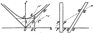
Sommerfeld (1909) – Spherical trigonometry

Using an imaginary rapidity such as Minkowski, Arnold Sommerfeld (1909) formulated a transformation equivalent to Lorentz boost (3b), and the relativistc velocity addition (4d) in terms of trigonometric functions and the spherical law of cosines:[R 44]

${\displaystyle {\begin{matrix}\left.{\begin{array}{lrl}x'=&x\ \cos \varphi +l\ \sin \varphi ,&y'=y\\l'=&-x\ \sin \varphi +l\ \cos \varphi ,&z'=z\end{array}}\right\}\\\left(\operatorname {tg} \varphi =i\beta ,\ \cos \varphi ={\frac {1}{\sqrt {1-\beta ^{2}}}},\ \sin \varphi ={\frac {i\beta }{\sqrt {1-\beta ^{2}}}}\right)\\\hline \beta ={\frac {1}{i}}\operatorname {tg} \left(\varphi _{1}+\varphi _{2}\right)={\frac {1}{i}}{\frac {\operatorname {tg} \varphi _{1}+\operatorname {tg} \varphi _{2}}{1-\operatorname {tg} \varphi _{1}\operatorname {tg} \varphi _{2}}}={\frac {\beta _{1}+\beta _{2}}{1+\beta _{1}\beta _{2}}}\\\cos \varphi =\cos \varphi _{1}\cos \varphi _{2}-\sin \varphi _{1}\sin \varphi _{2}\cos \alpha \\v^{2}={\frac {v_{1}^{2}+v_{2}^{2}+2v_{1}v_{2}\cos \alpha -{\frac {1}{c^{2}}}v_{1}^{2}v_{2}^{2}\sin ^{2}\alpha }{\left(1+{\frac {1}{c^{2}}}v_{1}v_{2}\cos \alpha \right)^{2}}}\end{matrix}}}$

Bateman and Cunningham (1909–1910) – Spherical wave transformation

In line with Lie's (1871) research on the relation between sphere transformations with an imaginary radius coordinate and 4D conformal transformations, it was pointed out by Bateman and Cunningham (1909–1910), that by setting u=ict as the imaginary fourth coordinates one can produce spacetime conformal transformations. Not only the quadratic form ${\displaystyle \lambda \left(dx^{2}+dy^{2}+dz^{2}+du^{2}\right)}$, but also Maxwells equations are covariant with respect to these transformations, irrespective of the choice of λ. These variants of conformal or Lie sphere transformations were called spherical wave transformations by Bateman.[R 45][R 46] However, this covariance is restricted to certain areas such as electrodynamics, whereas the totality of natural laws in inertial frames is covariant under the Lorentz group.[R 47] In particular, by setting λ=1 the Lorentz group SO(1,3) can be seen as a 10-parameter subgroup of the 15-parameter spacetime conformal group Con(1,3).

Bateman (1910/12)[89] also alluded to the identity between the Laguerre inversion and the Lorentz transformations. In general, the isomorphism between the Laguerre group and the Lorentz group was pointed out by Élie Cartan (1912, 1915/55),[24][R 48] Henri Poincaré (1912/21)[R 49] and others.

Herglotz (1909/10) – Möbius transformation

Following Klein (1889–1897) and Fricke & Klein (1897) concerning the Cayley absolute, hyperbolic motion and its transformation, Gustav Herglotz (1909/10) classified the one-parameter Lorentz transformations as loxodromic, hyperbolic, parabolic and elliptic. The general case (on the left) equivalent to Lorentz transformation (6a) and the hyperbolic case (on the right) equivalent to Lorentz transformation (3d) or squeeze mapping (9d) are as follows:[R 50]

${\displaystyle \left.{\begin{matrix}z_{1}^{2}+z_{2}^{2}+z_{3}^{2}-z_{4}^{2}=0\\z_{1}=x,\ z_{2}=y,\ z_{3}=z,\ z_{4}=t\\Z={\frac {z_{1}+iz_{2}}{z_{4}-z_{3}}}={\frac {x+iy}{t-z}},\ Z'={\frac {x'+iy'}{t'-z'}}\\Z={\frac {\alpha Z'+\beta }{\gamma Z'+\delta }}\end{matrix}}\right|{\begin{matrix}Z=Z'e^{\vartheta }\\{\begin{aligned}x&=x',&t-z&=(t'-z')e^{\vartheta }\\y&=y',&t+z&=(t'+z')e^{-\vartheta }\end{aligned}}\end{matrix}}}$

Varićak (1910) – Hyperbolic functions

Following Sommerfeld (1909), hyperbolic functions were used by Vladimir Varićak in several papers starting from 1910, who represented the equations of special relativity on the basis of hyperbolic geometry in terms of Weierstrass coordinates. For instance, by setting l=ct and v/c=tanh(u) with u as rapidity he wrote the Lorentz transformation in agreement with (3b):[R 51]

${\displaystyle {\begin{aligned}l'&=-x\operatorname {sh} u+l\operatorname {ch} u,\\x'&=x\operatorname {ch} u-l\operatorname {sh} u,\\y'&=y,\quad z'=z,\\\operatorname {ch} u&={\frac {1}{\sqrt {1-\left({\frac {v}{c}}\right)^{2}}}}\end{aligned}}}$

and showed the relation of rapidity to the Gudermannian function and the angle of parallelism:[R 51]

${\displaystyle {\frac {v}{c}}=\operatorname {th} u=\operatorname {tg} \psi =\sin \operatorname {gd} (u)=\cos \Pi (u)}$

He also related the velocity addition to the hyperbolic law of cosines:[R 52]

${\displaystyle {\begin{matrix}\operatorname {ch} {u}=\operatorname {ch} {u_{1}}\operatorname {c} h{u_{2}}+\operatorname {sh} {u_{1}}\operatorname {sh} {u_{2}}\cos \alpha \\\operatorname {ch} {u_{i}}={\frac {1}{\sqrt {1-\left({\frac {v_{i}}{c}}\right)^{2}}}},\ \operatorname {sh} {u_{i}}={\frac {v_{i}}{\sqrt {1-\left({\frac {v_{i}}{c}}\right)^{2}}}}\\v={\sqrt {v_{1}^{2}+v_{2}^{2}-\left({\frac {v_{1}v_{2}}{c}}\right)^{2}}}\ \left(a={\frac {\pi }{2}}\right)\end{matrix}}}$

Subsequently, other authors such as E. T. Whittaker (1910) or Alfred Robb (1911, who coined the name rapidity) used similar expressions, which are still used in modern textbooks.[10]

Ignatowski (1910)

While earlier derivations and formulations of the Lorentz transformation relied from the outset on optics, electrodynamics, or the invariance of the speed of light, Vladimir Ignatowski (1910) showed that it is possible to use the principle of relativity (and related group theoretical principles) alone, in order to derive the following transformation between two inertial frames:[R 53][R 54]

${\displaystyle {\begin{aligned}dx'&=p\ dx-pq\ dt\\dt'&=-pqn\ dx+p\ dt\\p&={\frac {1}{\sqrt {1-q^{2}n}}}\end{aligned}}}$

The variable n can be seen as a space-time constant whose value has to be determined by experiment or taken from a known physical law such as electrodynamics. For that purpose, Ignatowski used the above-mentioned Heaviside ellipsoid representing a contraction of electrostatic fields by x/γ in the direction of motion. It can be seen that this is only consistent with Ignatowski's transformation when n=1/c², resulting in p=γ and the Lorentz transformation (4b). With n=0, no length changes arise and the Galilean transformation follows. Ignatowski's method was further developed and improved by Philipp Frank and Hermann Rothe (1911, 1912),[R 55] with various authors developing similar methods in subsequent years.[90]

Noether (1910), Klein (1910) – Quaternions

Felix Klein (1908) described Cayley's (1854) 4D quaternion multiplications as "Drehstreckungen" (orthogonal substitutions in terms of rotations leaving invariant a quadratic form up to a factor), and pointed out that the modern principle of relativity as provided by Minkowski is essentially only the consequent application of such Drehstreckungen, even though he didn't provide details.[R 56]

In an appendix to Klein's and Sommerfeld's "Theory of the top" (1910), Fritz Noether showed how to formulate hyperbolic rotations using biquaternions with ${\displaystyle \omega ={\sqrt {-1}}}$, which he also related to the speed of light by setting ω²=-c². He concluded that this is the principal ingredient for a rational representation of the group of Lorentz transformations equivalent to (7a):[R 57]

${\displaystyle {\begin{matrix}V={\frac {Q_{1}vQ_{2}}{T_{1}T_{2}}}\\\hline X^{2}+Y^{2}+Z^{2}+\omega ^{2}S^{2}=x^{2}+y^{2}+z^{2}+\omega ^{2}s^{2}\\\hline {\begin{aligned}V&=Xi+Yj+Zk+\omega S\\v&=xi+yj+zk+\omega s\\Q_{1}&=(+Ai+Bj+Ck+D)+\omega (A'i+B'j+C'k+D')\\Q_{2}&=(-Ai-Bj-Ck+D)+\omega (A'i+B'j+C'k-D')\\T_{1}T_{2}&=T_{1}^{2}=T_{2}^{2}=A^{2}+B^{2}+C^{2}+D^{2}+\omega ^{2}\left(A^{\prime 2}+B^{\prime 2}+C^{\prime 2}+D^{\prime 2}\right)\end{aligned}}\end{matrix}}}$

Besides citing quaternion related standard works such as Cayley (1854), Noether referred to the entries in Klein's encyclopedia by Eduard Study (1899) and the French version by Élie Cartan (1908).[91] Cartan's version contains a description of Study's dual numbers, Clifford's biquaternions (including the choice ${\displaystyle \omega ={\sqrt {-1}}}$ for hyperbolic geometry), and Clifford algebra, with references to Stephanos (1883), Buchheim (1884/85), Vahlen (1901/02) and others.

Citing Noether, Klein himself published in August 1910 the following quaternion substitutions forming the group of Lorentz transformations:[R 58]

${\displaystyle {\begin{matrix}{\begin{aligned}&\left(i_{1}x'+i_{2}y'+i_{3}z'+ict'\right)\\&\quad -\left(i_{1}x_{0}+i_{2}y_{0}+i_{3}z_{0}+ict_{0}\right)\end{aligned}}={\frac {\left[{\begin{aligned}&\left(i_{1}(A+iA')+i_{2}(B+iB')+i_{3}(C+iC')+i_{4}(D+iD')\right)\\&\quad \cdot \left(i_{1}x+i_{2}y+i_{3}z+ict\right)\\&\quad \quad \cdot \left(i_{1}(A-iA')+i_{2}(B-iB')+i_{3}(C-iC')-(D-iD')\right)\end{aligned}}\right]}{\left(A^{\prime 2}+B^{\prime 2}+C^{\prime 2}+D^{\prime 2}\right)-\left(A^{2}+B^{2}+C^{2}+D^{2}\right)}}\\\hline {\text{where}}\\AA'+BB'+CC'+DD'=0\\A^{2}+B^{2}+C^{2}+D^{2}>A^{\prime 2}+B^{\prime 2}+C^{\prime 2}+D^{\prime 2}\end{matrix}}}$

or in March 1911[R 59]

${\displaystyle {\begin{matrix}g'={\frac {pg\pi }{M}}\\\hline {\begin{aligned}g&={\sqrt {-1}}ct+ix+jy+kz\\g'&={\sqrt {-1}}ct'+ix'+jy'+kz'\\p&=(D+{\sqrt {-1}}D')+i(A+{\sqrt {-1}}A')+j(B+{\sqrt {-1}}B')+k(C+{\sqrt {-1}}C')\\\pi &=(D-{\sqrt {-1}}D')-i(A-{\sqrt {-1}}A')-j(B-{\sqrt {-1}}B')-k(C-{\sqrt {-1}}C')\\M&=\left(A^{2}+B^{2}+C^{2}+D^{2}\right)-\left(A^{\prime 2}+B^{\prime 2}+C^{\prime 2}+D^{\prime 2}\right)\\&AA'+BB'+CC'+DD'=0\\&A^{2}+B^{2}+C^{2}+D^{2}>A^{\prime 2}+B^{\prime 2}+C^{\prime 2}+D^{\prime 2}\end{aligned}}\end{matrix}}}$

Conway (1911), Silberstein (1911) – Quaternions

Arthur W. Conway in February 1911 explicitly formulated quaternionic Lorentz transformations of various electromagnetic quantities in terms of velocity λ:[R 60]

${\displaystyle {\begin{matrix}{\begin{aligned}{\mathtt {D}}&=\mathbf {a} ^{-1}{\mathtt {D}}'\mathbf {a} ^{-1}\\{\mathtt {\sigma }}&=\mathbf {a} {\mathtt {\sigma }}'\mathbf {a} ^{-1}\end{aligned}}\\e=\mathbf {a} ^{-1}e'\mathbf {a} ^{-1}\\\hline a=\left(1-hc^{-1}\lambda \right)^{\frac {1}{2}}\left(1+c^{-2}\lambda ^{2}\right)^{-{\frac {1}{4}}}\end{matrix}}}$

Also Ludwik Silberstein in November 1911[R 61] as well as in 1914,[92] formulated the Lorentz transformation in terms of velocity v:

${\displaystyle {\begin{matrix}q'=QqQ\\\hline {\begin{aligned}q&=\mathbf {r} +l=xi+yj+zk+\iota ct\\q&'=\mathbf {r} '+l'=x'i+y'j+z'k+\iota ct'\\Q&={\frac {1}{\sqrt {2}}}\left({\sqrt {1+\gamma }}+\mathrm {u} {\sqrt {1-\gamma }}\right)\\&=\cos \alpha +\mathrm {u} \sin \alpha =e^{\alpha \mathrm {u} }\\&\left\{\gamma =\left(1-v^{2}/c^{2}\right)^{-1/2},\ 2\alpha =\operatorname {arctg} \ \left(\iota {\frac {v}{c}}\right)\right\}\end{aligned}}\end{matrix}}}$

Silberstein cites Cayley (1854, 1855) and Study's encyclopedia entry (in the extended French version of Cartan in 1908), as well as the appendix of Klein's and Sommerfeld's book.

Herglotz (1911), Silberstein (1911) – Vector transformation

Further information: Lorentz transformation § Vector transformations

Gustav Herglotz (1911)[R 62] showed how to formulate the transformation equivalent to (4c) in order to allow for arbitrary velocities and coordinates v=(v_x, v_y, v_z) and r=(x, y, z):

${\displaystyle {\begin{matrix}{\text{original}}&{\text{modern}}\\\hline \left.{\begin{aligned}x^{0}&=x+\alpha u(ux+vy+wz)-\beta ut\\y^{0}&=y+\alpha v(ux+vy+wz)-\beta vt\\z^{0}&=z+\alpha w(ux+vy+wz)-\beta wt\\t^{0}&=-\beta (ux+vy+wz)+\beta t\\&\alpha ={\frac {1}{{\sqrt {1-s^{2}}}\left(1+{\sqrt {1-s^{2}}}\right)}},\ \beta ={\frac {1}{\sqrt {1-s^{2}}}}\end{aligned}}\right|&{\begin{aligned}x'&=x+\alpha v_{x}\left(v_{x}x+v_{y}y+v_{z}z\right)-\gamma v_{x}t\\y'&=y+\alpha v_{y}\left(v_{x}x+v_{y}y+v_{z}z\right)-\gamma v_{y}t\\z'&=z+\alpha v_{z}\left(v_{x}x+v_{y}y+v_{z}z\right)-\gamma v_{z}t\\t'&=-\gamma \left(v_{x}x+v_{y}y+v_{z}z\right)+\gamma t\\&\alpha ={\frac {\gamma ^{2}}{\gamma +1}},\ \gamma ={\frac {1}{\sqrt {1-v^{2}}}}\end{aligned}}\end{matrix}}}$

This was simplified using vector notation by Ludwik Silberstein (1911 on the left, 1914 on the right):[R 63]

${\displaystyle {\begin{array}{c|c}{\begin{aligned}\mathbf {r} '&=\mathbf {r} +(\gamma -1)(\mathbf {ru} )\mathbf {u} +i\beta \gamma lu\\l'&=\gamma \left[l-i\beta (\mathbf {ru} )\right]\end{aligned}}&{\begin{aligned}\mathbf {r} '&=\mathbf {r} +\left[{\frac {\gamma -1}{v^{2}}}(\mathbf {vr} )-\gamma t\right]\mathbf {v} \\t'&=\gamma \left[t-{\frac {1}{c^{2}}}(\mathbf {vr} )\right]\end{aligned}}\end{array}}}$

Equivalent formulas were also given by Wolfgang Pauli (1921),[93] with Erwin Madelung (1922) providing the matrix form[94]

${\displaystyle {\begin{array}{c|c|c|c|c}&x&y&z&t\\\hline x'&1-{\frac {v_{x}^{2}}{v^{2}}}\left(1-{\frac {1}{\sqrt {1-\beta ^{2}}}}\right)&-{\frac {v_{x}v_{y}}{v^{2}}}\left(1-{\frac {1}{\sqrt {1-\beta ^{2}}}}\right)&-{\frac {v_{x}v_{z}}{v^{2}}}\left(1-{\frac {1}{\sqrt {1-\beta ^{2}}}}\right)&{\frac {-v_{x}}{\sqrt {1-\beta ^{2}}}}\\y'&-{\frac {v_{x}v_{y}}{v^{2}}}\left(1-{\frac {1}{\sqrt {1-\beta ^{2}}}}\right)&1-{\frac {v_{y}^{2}}{v^{2}}}\left(1-{\frac {1}{\sqrt {1-\beta ^{2}}}}\right)&-{\frac {v_{y}v_{z}}{v^{2}}}\left(1-{\frac {1}{\sqrt {1-\beta ^{2}}}}\right)&{\frac {-v_{y}}{\sqrt {1-\beta ^{2}}}}\\z'&-{\frac {v_{x}v_{z}}{v^{2}}}\left(1-{\frac {1}{\sqrt {1-\beta ^{2}}}}\right)&-{\frac {v_{y}v_{z}}{v^{2}}}\left(1-{\frac {1}{\sqrt {1-\beta ^{2}}}}\right)&1-{\frac {v_{z}^{2}}{v^{2}}}\left(1-{\frac {1}{\sqrt {1-\beta ^{2}}}}\right)&{\frac {-v_{z}}{\sqrt {1-\beta ^{2}}}}\\t'&{\frac {-v_{x}}{c^{2}{\sqrt {1-\beta ^{2}}}}}&{\frac {-v_{y}}{c^{2}{\sqrt {1-\beta ^{2}}}}}&{\frac {-v_{z}}{c^{2}{\sqrt {1-\beta ^{2}}}}}&{\frac {1}{\sqrt {1-\beta ^{2}}}}\end{array}}}$

These formulas were called "general Lorentz transformation without rotation" by Christian Møller (1952),[95] who in addition gave an even more general Lorentz transformation in which the Cartesian axes have different orientations, using a rotation operator ${\displaystyle {\mathfrak {D}}}$. In this case, v′=(v′_x, v′_y, v′_z) is not equal to -v=(-v_x, -v_y, -v_z), but the relation ${\displaystyle \mathbf {v} '=-{\mathfrak {D}}\mathbf {v} }$ holds instead, with the result

${\displaystyle {\begin{array}{c}{\begin{aligned}\mathbf {x} '&={\mathfrak {D}}^{-1}\mathbf {x} -\mathbf {v} '\left\{\left(\gamma -1\right)(\mathbf {x\cdot v} )/v^{2}-\gamma t\right\}\\t'&=\gamma \left(t-(\mathbf {v} \cdot \mathbf {x} )/c^{2}\right)\end{aligned}}\end{array}}}$

Borel (1913–14) – Cayley–Hermite parameter

Borel (1913) started by demonstrating Euclidean motions using Euler-Rodrigues parameter in three dimensions, and Cayley's (1846) parameter in four dimensions. Then he demonstrated the connection to indefinite quadratic forms expressing hyperbolic motions and Lorentz transformations. In three dimensions equivalent to (5b):[R 64]

${\displaystyle {\begin{matrix}x^{2}+y^{2}-z^{2}-1=0\\\hline {\scriptstyle {\begin{aligned}\delta a&=\lambda ^{2}+\mu ^{2}+\nu ^{2}-\rho ^{2},&\delta b&=2(\lambda \mu +\nu \rho ),&\delta c&=-2(\lambda \nu +\mu \rho ),\\\delta a'&=2(\lambda \mu -\nu \rho ),&\delta b'&=-\lambda ^{2}+\mu ^{2}+\nu ^{2}-\rho ^{2},&\delta c'&=2(\lambda \rho -\mu \nu ),\\\delta a''&=2(\lambda \nu -\mu \rho ),&\delta b''&=2(\lambda \rho +\mu \nu ),&\delta c''&=-\left(\lambda ^{2}+\mu ^{2}+\nu ^{2}+\rho ^{2}\right),\end{aligned}}}\\\left(\delta =\lambda ^{2}+\mu ^{2}-\rho ^{2}-\nu ^{2}\right)\\\lambda =\nu =0\rightarrow {\text{Hyperbolic rotation}}\end{matrix}}}$

In four dimensions equivalent to (5c):[R 65]

${\displaystyle {\begin{matrix}F=\left(x_{1}-x_{2}\right)^{2}+\left(y_{1}-y_{2}\right)^{2}+\left(z_{1}-z_{2}\right)^{2}-\left(t_{1}-t_{2}\right)^{2}\\\hline {\scriptstyle {\begin{aligned}&\left(\mu ^{2}+\nu ^{2}-\alpha ^{2}\right)\cos \varphi +\left(\lambda ^{2}-\beta ^{2}-\gamma ^{2}\right)\operatorname {ch} {\theta }&&-(\alpha \beta +\lambda \mu )(\cos \varphi -\operatorname {ch} {\theta })-\nu \sin \varphi -\gamma \operatorname {sh} {\theta }\\&-(\alpha \beta +\lambda \mu )(\cos \varphi -\operatorname {ch} {\theta })-\nu \sin \varphi +\gamma \operatorname {sh} {\theta }&&\left(\mu ^{2}+\nu ^{2}-\beta ^{2}\right)\cos \varphi +\left(\mu ^{2}-\alpha ^{2}-\gamma ^{2}\right)\operatorname {ch} {\theta }\\&-(\alpha \gamma +\lambda \nu )(\cos \varphi -\operatorname {ch} {\theta })+\mu \sin \varphi -\beta \operatorname {sh} {\theta }&&-(\beta \mu +\mu \nu )(\cos \varphi -\operatorname {ch} {\theta })+\lambda \sin \varphi +\alpha \operatorname {sh} {\theta }\\&(\gamma \mu -\beta \nu )(\cos \varphi -\operatorname {ch} {\theta })+\alpha \sin \varphi -\lambda \operatorname {sh} {\theta }&&-(\alpha \nu -\lambda \gamma )(\cos \varphi -\operatorname {ch} {\theta })+\beta \sin \varphi -\mu \operatorname {sh} {\theta }\\\\&\quad -(\alpha \gamma +\lambda \nu )(\cos \varphi -\operatorname {ch} {\theta })+\mu \sin \varphi +\beta \operatorname {sh} {\theta }&&\quad (\beta \nu -\mu \nu )(\cos \varphi -\operatorname {ch} {\theta })+\alpha \sin \varphi -\lambda \operatorname {sh} {\theta }\\&\quad -(\beta \mu +\mu \nu )(\cos \varphi -\operatorname {ch} {\theta })-\lambda \sin \varphi -\alpha \operatorname {sh} {\theta }&&\quad (\lambda \gamma -\alpha \nu )(\cos \varphi -\operatorname {ch} {\theta })+\beta \sin \varphi -\mu \operatorname {sh} {\theta }\\&\quad \left(\lambda ^{2}+\mu ^{2}-\gamma ^{2}\right)\cos \varphi +\left(\nu ^{2}-\alpha ^{2}-\beta ^{2}\right)\operatorname {ch} {\theta }&&\quad (\alpha \mu -\beta \lambda )(\cos \varphi -\operatorname {ch} {\theta })+\gamma \sin \varphi -\nu \operatorname {sh} {\theta }\\&\quad (\beta \gamma -\alpha \mu )(\cos \varphi -\operatorname {ch} {\theta })+\gamma \sin \varphi -\nu \operatorname {sh} {\theta }&&\quad -\left(\alpha ^{2}+\beta ^{2}+\gamma ^{2}\right)\cos \varphi +\left(\lambda ^{2}+\mu ^{2}+\nu ^{2}\right)\operatorname {ch} {\theta }\end{aligned}}}\\\left(\alpha ^{2}+\beta ^{2}+\gamma ^{2}-\lambda ^{2}-\mu ^{2}-\nu ^{2}=-1\right)\end{matrix}}}$

Gruner (1921) – Trigonometric Lorentz boosts

In order to simplify the graphical representation of Minkowski space, Paul Gruner (1921) (with the aid of Josef Sauter) developed what is now called Loedel diagrams, using the following relations:[R 66]

${\displaystyle {\begin{matrix}v=\alpha \cdot c;\quad \beta ={\frac {1}{\sqrt {1-\alpha ^{2}}}}\\\sin \varphi =\alpha$ ;\quad \beta ={\frac {1}{\cos \varphi }};\quad \alpha \beta =\tan \varphi \\\hline x'={\frac {x}{\cos \varphi }}-t\cdot \tan \varphi ,\quad t'={\frac {t}{\cos \varphi }}-x\cdot \tan \varphi \end{matrix}}}

This is equivalent to Lorentz transformation (8a) by the identity ${\displaystyle \sec \varphi ={\tfrac {1}{\cos \varphi }}}$

In another paper Gruner used the alternative relations:[R 67]

${\displaystyle {\begin{matrix}\alpha ={\frac {v}{c}};\ \beta ={\frac {1}{\sqrt {1-\alpha ^{2}}}};\\\cos \theta =\alpha ={\frac {v}{c}};\ \sin \theta ={\frac {1}{\beta }};\ \cot \theta =\alpha \cdot \beta \\\hline x'={\frac {x}{\sin \theta }}-t\cdot \cot \theta ,\quad t'={\frac {t}{\sin \theta }}-x\cdot \cot \theta \end{matrix}}}$

This is equivalent to Lorentz Lorentz boost (8b) by the identity ${\displaystyle \csc \theta ={\tfrac {1}{\sin \theta }}}$.

Euler's gap

In pursuing the history in years before Lorentz enunciated his expressions, one looks to the essence of the concept. In mathematical terms, Lorentz transformations are squeeze mappings, the linear transformations that turn a square into a rectangles of the same area. Before Euler, the squeezing was studied as quadrature of the hyperbola and led to the hyperbolic logarithm. In 1748 Euler issued his precalculus textbook where the number e is exploited for trigonometry in the unit circle. The first volume of Introduction to the Analysis of the Infinite had no diagrams, allowing teachers and students to draw their own illustrations.

There is a gap in Euler's text where Lorentz transformations arise. A feature of natural logarithm is its interpretation as area in hyperbolic sectors. In relativity the classical concept of velocity is replaced with rapidity, a hyperbolic angle concept built on hyperbolic sectors. A Lorentz transformation is a hyperbolic rotation which preserves differences of rapidity, just as the circular sector area is preserved with a circular rotation. Euler's gap is the lack of hyperbolic angle and hyperbolic functions, later developed by Johann H. Lambert. Euler described some transcendental functions: exponentiation and circular functions. He used the exponential series ${\displaystyle \sum _{0}^{\infty }x^{n}/n!.}$ With the imaginary unit i² = – 1, and splitting the series into even and odd terms, he obtained

${\displaystyle e^{ix}=\sum _{0}^{\infty }(ix)^{2n}/(2n)!\ +\ \sum _{0}^{\infty }(ix)^{2n+1}/(2n+1)!=}$

${\displaystyle =\sum _{0}^{\infty }(-1)^{n}x^{2n}/2n!+i\sum _{0}^{\infty }(-1)^{n}x^{2n+1}/(2n+1)!\ =\ \cos x+i\sin x.}$

This development misses the alternative:

${\displaystyle e^{x}=\cosh x+\sinh x}$ (even and odd terms), and

${\displaystyle e^{jx}=\cosh x+j\sinh x\quad (j^{2}=+1)}$ which parametrizes the unit hyperbola.

Here Euler could have noted split-complex numbers along with complex numbers.

For physics, one space dimension is insufficient. But to extend split-complex arithmetic to four dimensions leads to hyperbolic quaternions, and opens the door to abstract algebra's hypercomplex numbers. Reviewing the expressions of Lorentz and Einstein, one observes that the Lorentz factor is an algebraic function of velocity. For readers uncomfortable with transcendental functions cosh and sinh, algebraic functions may be more to their liking.

See also

• History of special relativity

References

Historical mathematical sources

1. Killing (1885), p. 71
2. Cayley (1884), section 16.
3. Klein (1896/97), p. 12
4. Kepler (1609), chapter 60. The editors of Kepler's collected papers remark (p. 482), that Kepler's relations correspond to ${\displaystyle {\scriptstyle \alpha =\beta +e\sin \beta }}$ and ${\displaystyle {\scriptstyle \cos \nu ={\frac {e+\cos \beta }{1+e\cos \beta }}}}$ and ${\displaystyle {\scriptstyle \cos \beta ={\frac {\cos \nu -e}{1-e\cos \nu }}}}$
5. Euler (1735/40), § 19
6. Euler (1748a), section VIII
7. Lagrange (1770/71), section I
8. Euler (1771), pp. 84-85
9. Euler (1771), pp. 77, 85-89
10. Rodrigues (1840), p. 405
11. Euler (1771), p. 101
12. Euler (1771), pp. 89–91
13. Euler (1748b), section 138.
14. Wessel (1799), § 28.
15. Riccati (1757), p. 71
16. Günther (1880/81), pp. 7–13
17. Lambert (1761/68), pp. 309–318
18. Lambert (1770), p. 335
19. Lagrange (1773/75), section 22
20. Gauss (1798/1801), articles 157–158;
21. Gauss (1798/1801), section 159
22. Gauss (1798/1801), articles 266–285
23. Gauss (1798/1801), article 277
24. Gauss (1800/1863), p. 311
25. Gauss (1818), pp. 5–10
26. Gauss (1818), pp. 9–10
27. Jacobi (1827), p. 235, 239–240
28. The orthogonal substitution and the imaginary transformation was defined in Jacobi (1832a), pp. 257, 265–267; Transformation system (2) and (3) and coefficients in Jacobi (1832b), pp. 321-325.
29. Jacobi (1833/34), pp. 7–8, 34–35, 41; Some misprints were corrected in Jacobi's collected papers, vol 3, pp. 229–230.
30. Jacobi (1833/34), p. 37. Some misprints were corrected in Jacobi's collected papers, vol 3, pp. 232–233.
31. Cauchy (1829), eq. 22, 98, 99, 101; Some misprints were corrected in Œuvres complètes, série 2, tome 9, pp. 174–195.
32. Lebesgue (1837), pp. 338-341
33. Lebesgue (1837), pp. 353–354
34. Lebesgue (1837), pp. 353–355
35. Hamilton (1844/45), p. 13
36. Hamilton (1844/45), p. 14
37. Cayley (1846)
38. Cayley (1855a), p. 288
39. Cayley (1858), p. 39
40. Cayley (1855b), p. 210
41. Cayley (1855b), p. 211
42. Cayley (1855b), pp. 212–213
43. Cayley (1854), p. 135
44. Fricke & Klein (1897), §12–13
45. Cayley (1879), p. 238f.
46. Helmholtz (1866/67), p. 513
47. Cayley (1845), p. 142
48. Cayley (1848), p. 196
49. Cayley (1854), p. 211
50. Cayley (1855b), p. 312
51. Cayley (1859), sections 209–229
52. Cockle (1848), p. 437
53. Cockle (1848), p. 438
54. Hermite (1853/54a), p. 307ff.
55. Hermite (1854b), p. 64
56. Frobenius (1877)
57. Hermite (1854b), pp. 64–65
58. Bour (1856), pp. 61; 64–65
59. Somov (1863), pp. 12–14; p. 18 for differentials.
60. Beltrami (1868a), pp. 287-288; Note I; Note II
61. Beltrami (1868b), pp. 232, 240–241, 253–254
62. Bachmann (1869), p. 303
63. Klein (1871), pp. 601–602
64. Klein (1871), p. 618
65. Klein (1873), pp. 127-128
66. Klein (1872), 6
67. Wedekind (1875), 1
68. Klein (1875), §1–2
69. Klein (1878), 8.
70. Klein (1882), p. 173.
71. Klein (1884), Part I, Ch. I, §1–2; Part II, Ch. II, 10
72. Klein (1893a), p. 109ff; pp. 138–140; pp. 249–250
73. Klein (1893b); general surface: pp. 61–66, 116–119, hyperbolic space: pp. 82, 86, 143–144
74. Klein (1896/97), pp. 13–14
75. Klein (1871/72), p. 268
76. Darboux (1872/73), p. 137
77. Lie (1871), p. 208
78. Pockels (1891), pp. 197–206
79. Klein (1893c), pp. 200ff (pentaspherical), pp. 373ff (tetracyclical)
80. Bôcher (1894), pp. 30–34, 40–43
81. Liouville (1847)
82. Euler (1777), p. 140
83. Lie (1871), pp. 199–209
84. Lie (1871a), pp. 199–209
85. Lie (1871/72), p. 186
86. Lie (1879/80), Collected papers, vol. 3, p. 389
87. Lie (1879/81), Collected papers, vol. 3, p. 393
88. Lie (1880/81), Collected papers, vol. 3, pp. 477–478
89. Lie (1883/84), Collected papers, vol. 3, p. 556
90. Lie (1885/86), p. 411
91. Werner (1889), pp. 4, 28
92. Lie (1890a), p. 295;
93. Lie (1890a), p. 311
94. Lie (1893), p. 474
95. Lie (1893), p. 479
96. Lie (1893), p. 481
97. Selling (1873), p. 174 and p. 179
98. Selling (1873), pp. 182–183
99. Selling (1873/74), p. 227 (see also p. 225 for citation).
100. Laisant (1874a), pp. 73–76
101. Laisant (1874b), pp. 134–135
102. Gudermann (1830), §1–3, §18–19
103. Escherich (1874), p. 508
104. Escherich (1874), p. 510
105. Cox (1881), p. 186
106. Glaisher (1878), p. 30
107. Killing (1877/78), p. 74; Killing (1880), p. 279
108. Killing (1880), eq. 25 on p. 283
109. Killing (1880), p. 283
110. Killing (1877/78), eq. 25 on p. 283
111. Killing (1879/80), p. 274
112. Killing (1885), pp. 18, 28–30, 53
113. Killing (1884/85), pp. 42–43; Killing (1885), pp. 73–74, 222
114. Killing (1884/85), pp. 4–5
115. Killing (1885), Note 9 on p. 260
116. Killing (1893), see pp. 144, 327–328
117. Killing (1893), pp. 314–316, 216–217
118. Killing (1893), p. 331
119. Killing (1898), p. 133
120. Killing (1887/88a), pp. 274–275
121. Killing (1892), p. 177
122. Killing (1897/98), pp. 255–256
123. Günther (1880/81), pp. 383–385
124. Günther (1880/81), p. 405
125. Poincaré (1881a), pp. 133–134
126. Poincaré (1881), pp. 133–134
127. Poincaré (1887), p. 206
128. Poincaré (1881b), p. 333
129. Poincaré (1883), pp. 49–50; 53–54
130. Poincaré (1886), p. 735ff.
131. Salmon (1862), section 212, p. 165
132. Frischauf (1876), pp. 86–87
133. Cox (1881), p. 186 for Weierstrass coordinates; (1881/82), pp. 193–194 for Lorentz transformation. On p. 193, the misprinted expression ${\displaystyle x^{2}-y^{2}-z^{2}}$ should read ${\displaystyle z^{2}-y^{2}-x^{2}}$
134. Cox (1881), pp. 199, 206–207
135. Cox (1881/82), p. 194
136. Cox (1882/83a), pp. 85–86
137. Cox (1882/83a), p. 88
138. Cox (1882/83b), p. 195
139. Cox (1882/83a), p. 97
140. On pp. 104-105 he started using the term v²=-1, on p. 106 he noted that one can simply use ${\displaystyle {\sqrt {-1}}}$ instead of v, and on p. 112 he adopted Clifford's notation by setting ω²=-1.
141. Cox (1882/83a), pp. 108-109
142. Hill (1882), pp. 323–325
143. Ribaucour (1870)
144. Laguerre (1882), pp. 550–551.
145. Picard (1882), pp. 307–308 first transformation system; pp. 315-317 second transformation system
146. Picard (1884a), p. 13
147. Picard (1884b), p. 416
148. Picard (1884c), pp. 123–124; 163
149. Stephanos (1883), p. 590ff
150. Stephanos (1883), p. 592
151. Buchheim (1885), p. 309
152. Darboux (1883), p. 849
153. Darboux (1891/94), pp. 381–382
154. Darboux (1887)
155. Callandreau (1885), pp. A.7; A.12
156. Lipschitz (1886), pp. 90–92
157. Lipschitz (1886), pp. 75–79
158. Lipschitz (1886), pp. 134–138
159. Lipschitz (1886), p. 76; p. 137
160. Lipschitz (1886), pp. 145–147
161. Schur (1885/86), p. 167
162. Schur (1900/02), p. 290; (1909), p. 83
163. Bianchi (1886), eq. 1 can be found on p. 226, eq. (2) on p. 240, eq. (3) on pp. 240–241, and for eq. (4) see the footnote on p. 240.
164. Bianchi (1894), pp. 433–434
165. Bianchi (1888), pp. 547; 562–563 (especially footnote on p. 563); 571–572
166. Bianchi (1893), § 3
167. Lindemann & Clebsch (1890/91), pp. 477–478, 524
168. Lindemann & Clebsch (1890/91), pp. 361–362
169. Lindemann & Clebsch (1890/91), p. 496
170. Lindemann & Clebsch (1890/91), pp. 477–478
171. Fricke (1891), §§ 1, 6
172. Fricke (1893), pp. 706, 710–711
173. Gérard (1892), pp. 40–41
174. Gérard (1892), pp. 40–41
175. Macfarlane (1892), p. 50; Macfarlane (1893), p. 24
176. Macfarlane (1894b), pp. 16–33
177. Macfarlane (1900), pp. 172, 175
178. Woods (1895), pp. 2–3; 10–11; 34–35
179. Woods (1901/02), p. 98, 104
180. Woods (1903/05), pp. 45–46; p. 48)
181. Woods (1903/05), p. 55
182. Woods (1903/05), p. 72
183. Whitehead (1898), pp. 459–460
184. Scheffers (1899), p. 158
185. Hausdorff (1899), p. 165, pp. 181-182
186. Hausdorff (1899), pp. 183-184
187. Smith (1900), p. 159
188. Vahlen (1902), pp. 586–587, 590; (1905), p. 282
189. Liebmann (1904/05), p. 168; pp. 175–176
190. Liebmann (1904/05), p. 174
191. Eisenhart (1905), p. 126

• Bachmann, P. (1869). "Zur Transformation der ternären quadratischen Formen". Journal für die Reine und Angewandte Mathematik. 71: 296–304.
• Beltrami, E. (1868a). "Saggio di interpretazione della geometria non-euclidea". Giornale di Matematiche. VI: 284–312. hdl:2027/ucm.5320603083.
• Beltrami, E. (1868b). "Teoria fondamentale degli spazii di curvatura costante". Annali di Matematica Pura ed Applicata. 2: 232–255. doi:10.1007/bf02419615.
• Bianchi, L. (1886). Lezioni di geometria differenziale. Pisa: Nistri.
• Bianchi, L. (1888). "Sulle forme differenziali quadratiche indefinite". Atti della R. Accademia dei Lincei. 4. 5: 539–603.
• Bianchi, L. (1893). "Ricerche sulle forme quaternarie quadratiche e sui gruppi poliedrici". Annali di Matematica Pura ed Applicata. 21 (1): 237–288. doi:10.1007/bf02420445. hdl:1908/1940.
• Bianchi, L. (1894). Lezioni di geometria differenziale. Pisa: Enrico Spoerri.
• Bôcher, M. (1894). Über die Reihenentwicklungen der Potentialtheorie. Leipzig: Macmillan.
• Bour, E. (1856) [1855]. "Sur l'attraction qu'exercerait une planètee". Journal de l'École Polytechnique. 36–38: 59–84.
• Buchheim, A. (1885) [1884]. "A memoir on biquaternions". American Journal of Mathematics. 7 (4): 293–326. doi:10.2307/2369176.
• Callandreau, O. (1882). "Calcul des variations seculaires des elements des orbites". Annales de l'Observatoire de Pari. 18: A.1–A.46. Bibcode:1885AnPar..18A...1C.
• Cauchy, A.L. (1829). "Sur l'équation à l'aide de laquelle on détermine les inégalités séculaires des mouvements des planètes". Exercises de Mathématiques. IV: 140–160.. Reprinted with corrections Œuvres complètes, série 2, tome 9.
• Cayley, A. (1845). "On certain Results relating to Quaternions". Philosophical Magazine. 26: 141–145. doi:10.1080/14786444508562684.
• Cayley, A. (1846). "Sur quelques propriétés des déterminants gauches". Journal für die Reine und Angewandte Mathematik. 32: 119–123.
• Cayley, A. (1848). "On the Application of Quaternions to the Theory of Rotation". Philosophical Magazine. 28: 196–200.
• Cayley, A. (1854). "On the homographic transformation of a surface of the second order into itself (continuation)". Philosophical Magazine. Series 44. 7 (44): 208–212. doi:10.1080/14786445408647451.
• Cayley, A. (1855a). "Sur la transformation d'une function quadratique en elle même par des substitutions linéaires". Journal für die Reine und Angewandte Mathematik. 50: 288–299.
• Cayley, A. (1855b). "Recherches ultérieurs sur les déterminants gauches". Journal für die Reine und Angewandte Mathematik. 50: 299–313.
• Cayley, A. (1858). "A memoir on the automorphic linear transformation of a bipartite quadric function". Philosophical Transactions of the Royal Society of London. 148: 39–46. doi:10.1098/rstl.1858.0003. JSTOR 108650.
• Cayley, A. (1859). "A sixth memoir upon quantics". Philosophical Transactions of the Royal Society of London. 149: 61–90. Bibcode:1859RSPT..149...61C. doi:10.1098/rstl.1859.0004. JSTOR 108690.
• Cayley, A. (1879). "On the correspondence of Homographies and Rotations". Mathematische Annalen. 15: 238–240. doi:10.1007/bf01444141.
• Cayley, A. (1884). "On the non-euclidian plane geometry". Proc. R. Soc. Lond. 37 (232–234): 82–102. doi:10.1098/rspl.1884.0018.
• Cockle, J. (1848). "On certain functions resembling quaternions, and on a new imaginary in algebra". Philosophical Magazine. Series 3 (224): 435–439.
• Cox, H. (1881). "Homogeneous coordinates in imaginary geometry and their application to systems of forces". The Quarterly Journal of Pure and Applied Mathematics. 18 (70): 178–192.
• Cox, H. (1882) [1881]. "Homogeneous coordinates in imaginary geometry and their application to systems of forces (continued)". The Quarterly Journal of Pure and Applied Mathematics. 18 (71): 193–215.
• Cox, H. (1883) [1882]. "On the Application of Quaternions and Grassmann's Ausdehnungslehre to different kinds of Uniform Space". Trans. Camb. Phil. Soc. 13: 69–143.
• Cox, H. (1883) [1882]. "On the Application of Quaternions and Grassmann's Ausdehnungslehre to different kinds of Uniform Space". Proc. Camb. Phil. Soc. 4: 194–196.
• Darboux, G. (1883). "Sur les surfaces dont la courbure totale est constante". Compt. Rend. 12: 848–850.
• Darboux, G. (1887). Leçons sur la théorie générale des surfaces. Première partie. Paris: Gauthier-Villars. pp. 254–256.
• Darboux, G. (1894) [1891]. Leçons sur la théorie générale des surfaces. Troisième partie. Paris: Gauthier-Villars. This third part of his lectures was initially published in three steps: première fascicule (1890), deuxième fascicule (1891), and troisième fascicule (1895). The discussion of the Lie transform appears in the deuxième fascicule published in 1891.
• Eisenhart, L. P. (1905). "Surfaces with the same Spherical Representation of their Lines of Curvature as Pseudospherical Surfaces". American Journal of Mathematics. 27 (2): 113–172. doi:10.2307/2369977.
• Escherich, G. von (1874). "Die Geometrie auf den Flächen constanter negativer Krümmung". Wiener Sitzungsberichte IIa. 69: 497–526.
• Euler, L. (1740) [1735]. "De motu planetarum et orbitarum determinatione". Novi Commentarii Academiae Scientiarum Petropolitanae. 7: 67–85.
• Euler, L. (1748a). "Memoire sur la plus grande equation des planetes". Memoires de l'academie des sciences de Berlin. 2: 225–248.
• Euler, L. (1748b). Introductio in analysin infinitorum, volume 1. Lausanne.
• Euler, L. (1771). "Problema algebraicum ob affectiones prorsus singulares memorabile". Novi Commentarii Academiae Scientiarum Petropolitanae. 15: 75–106.
• Euler, L. (1777). "De proiectione geographica superficiei sphaericae". Acta Academiae Scientiarum Imperialis Petropolitanae: 133–142.
• Fricke, R. (1891). "Ueber eine besondere Classe discontinuirlicher Gruppen reeller linearer Substitutionen". Mathematische Annalen. 38: 50–81. doi:10.1007/bf01212693.
• Fricke, R. (1893). "Ueber indefinite quadratische Formen mit drei und vier Veränderlichen". Gött. Nachr.: 705–721.
• Fricke R.; Klein, F. (1897). Vorlesungen über die Theorie der automorphen Functionen – Erster Band: Die gruppentheoretischen Grundlagen. Leipzig: Teubner.
• Frischauf, J. (1876). Elemente der absoluten Geometrie. Leipzig: Teubner.
• Frobenius, G. (1877). "Ueber lineare Substitutionen und bilineare Formen". Journal für die Reine und Angewandte Mathematik. 84: 1–63.
• Gauss, C.F (1801) [1798]. Disquisitiones arithmeticae. Leipzig: Fleischer.
• Gauss, C.F. (1863) [1800]. Werke – Zweiter Band. Göttingen.
• Gauss, C.F. (1818). Determinatio attractionis, quam in punctum quodvis positionis datae exerceret planet. Göttingen: Dietrich. doi:10.3931/e-rara-8856.
• Gérard, L. (1892). Sur la géométrie non-Euclidienne. Paris: Gauthier-Villars.
• Glaisher, JWL (1878). "On a special form of determinant, and on ceetain functions of n variables analogous to the sine and cosine". The Quarterly Journal of Pure and Applied Mathematics. 16: 15–33.
• Gudermann, C. (1830). Grundriss der analytischen Sphärik. Cologne: DüMont-Schauberg.
• Günther, S. (1881) [1880]. Die Lehre von den gewöhnlichen und verallgemeinerten Hyperbelfunktionen. Halle: L. Nebert.
• Hamilton, W.R. (1847) [1844]. "On Quaternions". Proceedings of the Royal Irish Academy. III (48): 1–16. – Issue 48 for 1844-1845, full volume III published in 1847.
• Hausdorff, F. (1899). "Analytische Beiträge zur nichteuklidischen Geometrie". Leipziger Math.-Phys. Berichte. 51: 161–214. hdl:2027/hvd.32044092889328.
• Helmholtz, H. von (1867) [1866]. Handbuch der physiologischen Optik. Leipzig: Voss.
• Hermite, C. (1854a) [1853]. "Sur la théorie des formes quadratiques ternaires indéfinies". Journal für die Reine und Angewandte Mathematik. 47: 307–312.
• Hermite, C. (1854b). "Remarques sur un memoire de M. Cayley relatif aux determinants gauches". The Cambridge and Dublin Mathematical Journal. 9: 63–67.
• Hill, G. W. (1882). "On Gauss's Method of Computing Secular Perturbations". Astronomical Papers of the American Ephemeris. I: 315–361.
• Jacobi, C.G.J. (1827). "De singulari quadam duplicis Integeralis transformatione". Journal für die Reine und Angewandte Mathematik. 2: 234–242.
• Jacobi, C.G.J. (1832a). "De transformatione integralis duplicis indefinit..." Journal für die Reine und Angewandte Mathematik. 8: 253–279.
• Jacobi, C.G.J. (1832b). "De transformatione integralis duplicis indefinit..." Journal für die Reine und Angewandte Mathematik. 8: 321–357.
• Jacobi, C.G.J. (1834) [1833]. "De binis quibuslibet functionibus homogeneis secundi ordinis per substitutiones lineares..." Journal für die Reine und Angewandte Mathematik. 12: 1–69.. All papers (1827, 1832a, 1832b, 1834) were reprinted with corrections in Jacobi's collected papers vol. 3.
• Kepler, J. (1609). Astronomia nova. Heidelberg: Voegelin. doi:10.3931/e-rara-558.. Reprinted with corrections and comments in Kepler's collected papers vol. 3.
• Killing, W. (1878) [1877]. "Ueber zwei Raumformen mit constanter positiver Krümmung". Journal für die Reine und Angewandte Mathematik. 86: 72–83.
• Killing, W. (1880) [1879]. "Die Rechnung in den Nicht-Euklidischen Raumformen". Journal für die Reine und Angewandte Mathematik. 89: 265–287.
• Killing, W. (1885) [1884]. "Die Mechanik in den Nicht-Euklidischen Raumformen". Journal für die Reine und Angewandte Mathematik. 98: 1–48.
• Killing, W. (1885). Die nicht-euklidischen Raumformen. Leipzig: Teubner.
• Killing, W. (1893). Einführung in die Grundlagen der Geometrie I. Paderborn: Schöningh.
• Killing, W. (1898) [1897]. Einführung in die Grundlagen der Geometrie II. Paderborn: Schöningh.
• Klein, F. (1871). "Ueber die sogenannte Nicht-Euklidische Geometrie". Mathematische Annalen. 4: 573–625. doi:10.1007/bf02100583.
• Klein, F. (1872) [1871]. "Ueber Liniengeometrie und metrische Geometrie". Mathematische Annalen. 5: 257–277. doi:10.1007/bf01444841.
• Klein, F. (1872). Vergleichende Betrachtungen über neuere geometrische Forschungen. Erlangen: Deichert.
• Klein, F. (1873). "Ueber die sogenannte Nicht-Euklidische Geometrie". Mathematische Annalen. 6: 112–145. doi:10.1007/bf01443189.
• Klein, F. (1875). "Ueber binäre Formen mit linearen Transformationen in sich selbst". Mathematische Annalen. 9: 183–208. doi:10.1007/bf01443373.
• Klein, F. (1879) [1878]. "Ueber die Transformation der elliptischen Functionen und die Auflösung der Gleichungen fünften Grades". Mathematische Annalen. 14: 111–172. doi:10.1007/bf02297507.
• Klein, F. (1883) [1882]. "Neue Beiträge zur Riemann'schen Functionentheorie". Mathematische Annalen. 21: 141–218. doi:10.1007/bf01442920.
• Klein, F. (1884). Vorlesungen über das Ikosaeder und die Auflösung der Gleichungen vom fünften Grade. Leipzig: Teubner.; English translation: Lectures on the ikosahedron and the solution of equations of the fifth degree (1888)
• Klein, F.; Fricke, R. (1890a). Vorlesungen über die Theorie der elliptische Modulfunctionen. Leipzig: Teubner.
• Klein, F. (1890b). "Zur Nicht-Euklidischen Geometrie". Mathematische Annalen. 37: 544–572. doi:10.1007/bf01724772.
• Klein, F. (1893a) [1890]. Schilling, Fr. (ed.). Nicht-Euklidische Geometrie I, Vorlesung gehalten während des Wintersemesters 1889–90. Göttingen: Göttingen.
• Klein, F. (1893b) [1890]. Schilling, Fr. (ed.). Nicht-Euklidische Geometrie II, Vorlesung gehalten während des Sommersemesters 1890. Göttingen: Göttingen.
• Klein, F. (1893c). Schilling, Fr. (ed.). Einleitung in die höhere Geometrie I, Vorlesung gehalten während des Wintersemesters 1892–93. Göttingen.
• Klein, F. (1893d). Schilling, Fr. (ed.). Einleitung in die höhere Geometrie II, Vorlesung gehalten während des Sommersemesters 1893. Göttingen.
• Klein, F. (1897) [1896]. The Mathematical Theory of the Top. New York: Scribner.
• Lagrange, J. L. (1771) [1770]. "Sur le Problème de Kepler". Nouveaux Mémoires de l'Académie Royale des Sciences et Belles-Lettres de Berlin: 204–233.
• Lagrange, J. L. (1775) [1773]. "Recherches d'arithmetique". Nouveaux Mémoires de l'Académie Royale des Sciences et Belles-Lettres de Berlin: 265–314.
• Laguerre, Edmond (1881). "Sur la transformation par directions réciproques". Comptes Rendus. 92: 71–73.
• Laguerre, Edmond (1882). "Transformations par semi-droites réciproques" . Nouvelles annales de mathématiques. 1: 542–556.
• Laisant, C. A. (1874a). Essai sur les fonctions hyperboliques. Gauthier-Villars.
• Laisant, C. A. (1874b) [1854]. "Étude de l'hyperbole". French translation of Giusto Bellavitis (1854), Exposition de la méthode des equipollences. Gauthier-Villars. pp. 133–136.
• Lambert, J. H. (1768) [1767]. "Mémoire sur quelques propriétés remarquables des quantités transcendentes circulaires et logarithmiques". Histoire de l'Académie Royale des Sciences et des Belles-Lettres de Berlin. 17: 265–322.
• Lambert, J. H. (1770). "Observations trigonométriques". Histoire de l'Académie Royale des Sciences et des Belles-Lettres de Berlin. 24: 327–354.
• Lebesgue, V.A. (1837). "Thèses de Mécanique et d'Astronomie" (PDF). Journal de Mathématiques Pures et Appliquées. 1. 2: 1–69.
• Lie, S. (1871a). "Ueber diejenige Theorie eines Raumes mit beliebig vielen Dimensionen, die der Krümmungs-Theorie des gewöhnlichen Raumes entspricht". Göttinger Nachrichten: 191–209.
• Lie, S. (1872) [1871]. "Ueber Complexe, insbesondere Linien- und Kugel-Complexe, mit Anwendung auf die Theorie partieller Differentialgleichungen". Mathematische Annalen. 5: 145–256. doi:10.1007/bf01446331. English translation by David Delphenich: On complexes – in particular, line and sphere complexes – with applications to the theory of partial differential equations
• Lie, S. (1880) [1879]. "Über Flächen, deren Krümmungsradien durch eine Relation verknüpft sind". Archiv for Mathematik. 4 (4): 507–512. Reprinted in Lie's collected papers, Vol. 3, pp. 387–391.
• Lie, S. (1881) [1879]. "Selbstanzeige: Über Flächen, deren Krümmungsradien durch eine Relation verknüpft sind". Fortschritte der Matheamtik. 11: 529–531. Reprinted in Lie's collected papers, Vol. 3, pp. 392–393.
• Lie, S. (1881) [1880]. "Diskussion der Differentialgleichung d2dz/dxdy". Archiv for Mathematik. 6 (1): 112–124. Reprinted in Lie's collected papers, Vol. 3, pp. 469–478.
• Lie, S. (1884) [1883]. "Untersuchungen über Differentialgleichungen IV". Christ. Forh. Reprinted in Lie's collected papers, Vol. 3, pp. 556–560.
• Lie, Sophus (1886) [1885]. "Untersuchungen über Transformationsgruppen II". Archiv for Mathematik og Naturvidenskab. 10 (4): 353–413.
• Lie, S. (1890). "Ueber die Grundlagen der Geometrie I". Leipz. Ber.: 284–321.
• Lie, S. (1893). Theorie der Transformationsgruppen (Dritter und letzter Abschnitt, unter Mitwirkung von Prof. Dr. Friedrich Engel). Leipzig: Leipzig, B.G. Teubner.
• Liebmann, H. (1905) [1904]. Nichteuklidische Geometrie. Leipzig: Göschen.
• Lindemann, F.; Clebsch, A. (1891) [1890]. Vorlesungen über Geometrie von Clebsch II. Leipzig: Teubner.
• Liouville, Joseph (1850). "Théorème sur l'équation dx²+dy²+dz²=λ(dα²+dβ²+dγ²)". Journal de Mathématiques Pures et Appliquées. 15: 103.
• Lipschitz, R. (1886). Untersuchungen ueber die Summen von Quadraten. Bonn: Cohen.
• Macfarlane, A. (1892). "The Imaginary of Algebra". Proceedings of the American Association for the Advancement of Science. 41: 33–55.
• Macfarlane, A. (1893). The Fundamental Theorems of Analysis Generalized for Space. Boston: Cushing.
• Macfarlane, A. (1894). The principles of elliptic and hyperbolic analysis. Boston: Boston, J.S. Cushing & co., printers.
• Macfarlane, A. (1902) [1900]. "Hyperbolic quaternions". Proceedings of the Royal Society of Edinburgh. 23: 169–180. doi:10.1017/s0370164600010385.
• Picard, E. (1882). "Sur une classe de groupes discontinus de substitutions linéaires et sur les fonctions de deux variables indépendantes restant invariables par ces substitutions". Acta Mathematica. 1: 297–320. doi:10.1007/BF02592137.
• Picard, E. (1884a). "Mémoire sur les formes quadratiques binaires indéfinies à indéterminées conjuguées". Annales Scientifiques de l'École Normale Supérieure. 1: 9–54. doi:10.24033/asens.231.
• Picard, E. (1884b). "Sur certaines substitutions lineaires". Comptes Rendus. 98: 416–417.
• Picard, E. (1884c). "Sur les formes quadratiques ternaires indéfinies á indéterminées conjuguées et sur les fonctions hyperfuchsiennes correspondantes". Acta Mathematica. 5: 121–182. doi:10.1007/BF02421555.
• Pockels, F. (1891). Über die partielle Differentialgleichung Δu+k²u=0 und deren Auftreten in der mathematischen Physik. Leipzig: Teubner.
• Poincaré, H. (1881a). "Sur les applications de la géométrie non-euclidienne à la théorie des formes quadratiques" (PDF). Association Française Pour l'Avancement des Sciences. 10: 132–138.
• Poincaré, H. (1881b). "Sur les fonctions fuchsiennes" (PDF). Comptes Rendus Hebdomadaires des Séances de l'Académie des Sciences. 92: 333–335.
• Poincaré, H. (1883). "Mémoire sur les groupes kleinéens" (PDF). Acta Mathematica. 3: 49–92. doi:10.1007/bf02422441.
• Poincaré, H. (1886). "Sur les fonctions fuchsiennes et les formes quadratiques ternaires indéfinies" (PDF). Comptes Rendus Hebdomadaires des Séances de l'Académie des Sciences. 102: 735–737.
• Poincaré, H. (1887). "Sur les hypothèses fondamentales de la géométrie" (PDF). Bulletin de la Société Mathématique de France. 15: 203–216.
• Ribaucour, Albert (1870). "Sur la déformation des surfaces". Comptes Rendus. 70: 330–333.
• Riccati, V. (1757). Opusculorum ad res physicas, et mathematicas pertinentium. Aquinatis.
• Rodrigues, O. (1840). "Des lois géométriques qui régissent les déplacements d'un système solide dans l'espace". Journal de Mathématiques Pures et Appliquées. 5: 380–440.
• Salmon, G. (1862). A Treatise on the Analytic Geometry of Three Dimensions. Dublin.
• Scheffers, G. (1899). "Synthetische Bestimmung aller Berührungstransformationen der Kreise in der Ebene". Leipziger Math.-Phys. Berichte. 51: 145–160. hdl:2027/hvd.32044092889328.
• Schur, F. (1886) [1885]. "Ueber die Deformation der Räume constanten Riemann'schen Krümmungsmaasses". Mathematische Annalen. 27: 163–176.
• Schur, F. (1902) [1900]. "Ueber die Grundlagen der Geometrie". Mathematische Annalen. 55: 265–292. doi:10.1007/bf01444974.
• Schur, F. (1909). Grundlagen der Geometrie. Leipzig: Teubner.
• Selling, Eduard (1874) [1873]. "Ueber die binären und ternären quadratischen Formen". Journal für die Reine und Angewandte Mathematik. 77: 143–229.
• Smith, Percey F. (1900). "On a Transformation of Laguerre". Annals of Mathematics. 1 (1/4): 153–172. doi:10.2307/1967282. JSTOR 1967282.
• Somov, I. (1863). "Mémoire sur un cas particulier de l'homographie". Mémoires de l'Acad. Imp. Des Sciences de St.-Petersbourg. 7. 5 (9).
• Stephanos, C. (1883). "Sur la théorie des quaternions". Mathematische Annalen. 7 (4): 589–592. doi:10.1007/bf01443267.
• Taurinus, Franz Adolph (1826). Geometriae prima elementa. Recensuit et novas observationes adjecit. Köln: Bachem.; Partial German translation: Taurinus, Franz Adolph (1895) [1826]. "Geometriae. Prima elementa. Recensuit et novas observationes adjecit". In Engel, F; Stäckel, P. (eds.). Die Theorie der Parallellinien von Euklid bis auf Gauss. Leipzig: Teubner. pp. 267–286.
• Vahlen, K.Th. (1902) [1901]. "Ueber Bewegungen und complexe Zahlen". Mathematische Annalen. 55: 585–593. doi:10.1007/bf01450354.
• Vahlen, K.Th. (1905). Abstrakte Geometrie. Leipzig: Teubner.
• Wedekind, L. (1875). Beiträge zur geometrischen Interpretation binärer Formen. Erlangen.
• Werner, H. (1889). Bestimmung der grössten Untergruppen derjenigen projectiven Gruppe, welche eine Gleichung zweiten Grades in n Veränderlichen invariant lässt. Leipzig: Teubner.
• Wessel, C. (1799) [1797]. "Om directionens analytiske betegning". Royal Danish Academy of Sciences and Letters. 7 (4): 469–518.; French translation (1897): Essai sur la représentation analytique de la direction
• Whitehead, A. (1898). A Treatise on Universal Algebra. Cambridge University Press.
• Woods, F. S. (1895). Ueber Pseudominimalflächen. Göttingen: Kästner. hdl:2027/uc1.b2620512.
• Woods, F. S. (1901). "Space of constant curvature". The Annals of Mathematics. 3 (1/4): 71–112. JSTOR 1967636.
• Woods, F. S. (1905) [1903]. "Forms of non-Euclidean space". The Boston Colloquium: Lectures on Mathematics for the Year 1903: 31–74.

Historical relativity sources

1. Varićak (1912), p. 108
2. Borel (1914), pp. 39–41
3. Brill (1925)
4. Voigt (1887), p. 45
5. Lorentz (1915/16), p. 197
6. Lorentz (1915/16), p. 198
7. Bucherer (1908), p. 762
8. Heaviside (1888), p. 324
9. Thomson (1889), p. 12
10. Searle (1886), p. 333
11. Lorentz (1892a), p. 141
12. Lorentz (1892b), p. 141
13. Lorentz (1895), p. 37
14. Lorentz (1895), p. 49 for local time and p. 56 for spatial coordinates.
15. Larmor (1897), p. 229
16. Larmor (1897/1929), p. 39
17. Larmor (1900), p. 168
18. Larmor (1900), p. 174
19. Larmor (1904a), p. 583, 585
20. Larmor (1904b), p. 622
21. Lorentz (1899), p. 429
22. Lorentz (1899), p. 439
23. Lorentz (1899), p. 442
24. Lorentz (1904), p. 812
25. Lorentz (1904), p. 826
26. Bucherer, p. 129; Definition of s on p. 32
27. Wien (1904), p. 394
28. Cohn (1904a), pp. 1296-1297
29. Gans (1905), p. 169
30. Poincaré (1900), pp. 272–273
31. Cohn (1904b), p. 1408
32. Abraham (1905), § 42
33. Poincaré (1905), p. 1505
34. Poincaré (1905/06), pp. 129ff
35. Poincaré (1905/06), p. 144
36. Einstein (1905), p. 902
37. Einstein (1905), § 5 and § 9
38. Einstein (1905), § 7
39. Minkowski (1907/15), pp. 927ff
40. Minkowski (1907/08), pp. 53ff
41. Minkowski (1907/08), p. 59
42. Minkowski (1907/08), pp. 65–66, 81–82
43. Minkowski (1908/09), p. 77
44. Sommerfeld (1909), p. 826ff.
45. Bateman (1909/10), pp. 223ff
46. Cunningham (1909/10), pp. 77ff
47. Klein (1910)
48. Cartan (1912), p. 23
49. Poincaré (1912/21), p. 145
50. Herglotz (1909/10), pp. 404-408
51. Varićak (1910), p. 93
52. Varićak (1910), p. 94
53. Ignatowski (1910), pp. 973–974
54. Ignatowski (1910/11), p. 13
55. Frank & Rothe (1911), pp. 825ff; (1912), p. 750ff.
56. Klein (1908), p. 165
57. Noether (1910), pp. 939–943
58. Klein (1910), p. 300
59. Klein (1911), pp. 602ff.
60. Conway (1911), p. 8
61. Silberstein (1911/12), p. 793
62. Herglotz (1911), p. 497
63. Silberstein (1911/12), p. 792; (1914), p. 123
64. Borel (1913/14), p. 39
65. Borel (1913/14), p. 41
66. Gruner (1921a),
67. Gruner (1921b)

• Abraham, M. (1905). "§ 42. Die Lichtzeit in einem gleichförmig bewegten System" . Theorie der Elektrizität: Elektromagnetische Theorie der Strahlung. Leipzig: Teubner.
• Bateman, Harry (1910) [1909]. "The Transformation of the Electrodynamical Equations" . Proceedings of the London Mathematical Society. 8: 223–264. doi:10.1112/plms/s2-8.1.223.
• Bateman, Harry (1912) [1910]. "Some geometrical theorems connected with Laplace's equation and the equation of wave motion". American Journal of Mathematics. 34 (3): 325–360. doi:10.2307/2370223. JSTOR 2370223.
• Borel, Émile (1914). Introduction Geometrique à quelques Théories Physiques. Paris.
• Brill, J. (1925). "Note on the Lorentz group". Proceedings of the Cambridge Philosophical Society. 22 (5): 630. Bibcode:1925PCPS...22..630B. doi:10.1017/S030500410000949X.
• Bucherer, A. H. (1904). Mathematische Einführung in die Elektronentheorie. Leipzig: Teubner.
• Bucherer, A. H. (1908), "Messungen an Becquerelstrahlen. Die experimentelle Bestätigung der Lorentz-Einsteinschen Theorie. (Measurements of Becquerel rays. The Experimental Confirmation of the Lorentz-Einstein Theory)", Physikalische Zeitschrift, 9 (22): 758–762. For Minkowski's and Voigt's statements see p. 762.
• Cartan, Élie (1912). "Sur les groupes de transformation de contact et la Cinématique nouvelle". Société de Mathématique the France – Comptes Rendus des Séances: 23.
• Cohn, Emil (1904a), "Zur Elektrodynamik bewegter Systeme I" [On the Electrodynamics of Moving Systems I], Sitzungsberichte der Königlich Preussischen Akademie der Wissenschaften, 1904/2 (40): 1294–1303
• Cohn, Emil (1904b), "Zur Elektrodynamik bewegter Systeme II" [On the Electrodynamics of Moving Systems II], Sitzungsberichte der Königlich Preussischen Akademie der Wissenschaften, 1904/2 (43): 1404–1416
• Conway, A. W. (1911). "On the application of quaternions to some recent developments of electrical theory". Proceedings of the Royal Irish Academy, Section A. 29: 1–9.
• Cunningham, Ebenezer (1910) [1909]. "The principle of Relativity in Electrodynamics and an Extension Thereof" . Proceedings of the London Mathematical Society. 8: 77–98. doi:10.1112/plms/s2-8.1.77.
• Einstein, Albert (1905), "Zur Elektrodynamik bewegter Körper" (PDF), Annalen der Physik, 322 (10): 891–921, Bibcode:1905AnP...322..891E, doi:10.1002/andp.19053221004. See also: English translation.
• Frank, Philipp; Rothe, Hermann (1911). "Über die Transformation der Raum-Zeitkoordinaten von ruhenden auf bewegte Systeme". Annalen der Physik. 339 (5): 825–855. Bibcode:1911AnP...339..825F. doi:10.1002/andp.19113390502.
• Frank, Philipp; Rothe, Hermann (1912). "Zur Herleitung der Lorentztransformation". Physikalische Zeitschrift. 13: 750–753.
• Gans, Richard (1905), "H. A. Lorentz. Elektromagnetische Vorgänge" [H.A. Lorentz: Electromagnetic Phenomena], Beiblätter zu den Annalen der Physik, 29 (4): 168–170
• Gruner, Paul & Sauter, Josef (1921a). "Représentation géométrique élémentaire des formules de la théorie de la relativité" [Elementary geometric representation of the formulas of the special theory of relativity]. Archives des sciences physiques et naturelles. 5. 3: 295–296.
• Gruner, Paul (1921b). "Eine elementare geometrische Darstellung der Transformationsformeln der speziellen Relativitätstheorie" [An elementary geometrical representation of the transformation formulas of the special theory of relativity]. Physikalische Zeitschrift. 22: 384–385.
• Heaviside, Oliver (1889), "On the Electromagnetic Effects due to the Motion of Electrification through a Dielectric" (PDF), Philosophical Magazine, 5, 27 (167): 324–339, doi:10.1080/14786448908628362
• Herglotz, Gustav (1910) [1909], "Über den vom Standpunkt des Relativitätsprinzips aus als starr zu bezeichnenden Körper" [Wikisource translation: On bodies that are to be designated as "rigid" from the standpoint of the relativity principle], Annalen der Physik, 336 (2): 393–415, Bibcode:1910AnP...336..393H, doi:10.1002/andp.19103360208
• Herglotz, G. (1911). "Über die Mechanik des deformierbaren Körpers vom Standpunkte der Relativitätstheorie". Annalen der Physik. 341 (13): 493–533. Bibcode:1911AnP...341..493H. doi:10.1002/andp.19113411303.; English translation by David Delphenich: On the mechanics of deformable bodies from the standpoint of relativity theory.
• Ignatowsky, W. v. (1910). "Einige allgemeine Bemerkungen über das Relativitätsprinzip" . Physikalische Zeitschrift. 11: 972–976.
• Ignatowski, W. v. (1911) [1910]. "Das Relativitätsprinzip" . Archiv der Mathematik und Physik. 18: 17–40.
• Ignatowski, W. v. (1911). "Eine Bemerkung zu meiner Arbeit: "Einige allgemeine Bemerkungen zum Relativitätsprinzip"" . Physikalische Zeitschrift. 12: 779.
• Klein, F. (1908). Hellinger, E. (ed.). Elementarmethematik vom höheren Standpunkte aus. Teil I. Vorlesung gehalten während des Wintersemesters 1907-08. Leipzig: Teubner.
• Klein, Felix (1921) [1910]. Über die geometrischen Grundlagen der Lorentzgruppe . Gesammelte Mathematische Abhandlungen. 1. pp. 533–552. doi:10.1007/978-3-642-51960-4_31. ISBN 978-3-642-51898-0.
• Klein, F.; Sommerfeld A. (1910). Noether, Fr. (ed.). Über die Theorie des Kreisels. Heft IV. Leipzig: Teuber.
• Klein, F. (1911). Hellinger, E. (ed.). Elementarmethematik vom höheren Standpunkte aus. Teil I (Second Edition). Vorlesung gehalten während des Wintersemesters 1907-08. Leipzig: Teubner. hdl:2027/mdp.39015068187817.
• Larmor, Joseph (1897), "On a Dynamical Theory of the Electric and Luminiferous Medium, Part 3, Relations with material media" , Philosophical Transactions of the Royal Society, 190: 205–300, Bibcode:1897RSPTA.190..205L, doi:10.1098/rsta.1897.0020
• Larmor, Joseph (1929) [1897], "On a Dynamical Theory of the Electric and Luminiferous Medium. Part 3: Relations with material media", Mathematical and Physical Papers: Volume II, Cambridge University Press, pp. 2–132, ISBN 978-1-107-53640-1 (Reprint of Larmor (1897) with new annotations by Larmor.)
• Larmor, Joseph (1900), Aether and Matter , Cambridge University Press
• Larmor, Joseph (1904a). "On the intensity of the natural radiation from moving bodies and its mechanical reaction". Philosophical Magazine. 7 (41): 578–586. doi:10.1080/14786440409463149.
• Larmor, Joseph (1904b). "On the ascertained Absence of Effects of Motion through the Aether, in relation to the Constitution of Matter, and on the FitzGerald-Lorentz Hypothesis" . Philosophical Magazine. 7 (42): 621–625. doi:10.1080/14786440409463156.
• Lorentz, Hendrik Antoon (1892a), "La Théorie electromagnétique de Maxwell et son application aux corps mouvants", Archives Néerlandaises des Sciences Exactes et Naturelles, 25: 363–552
• Lorentz, Hendrik Antoon (1892b), "De relatieve beweging van de aarde en den aether" [The Relative Motion of the Earth and the Aether], Zittingsverlag Akad. V. Wet., 1: 74–79
• Lorentz, Hendrik Antoon (1895), Versuch einer Theorie der electrischen und optischen Erscheinungen in bewegten Körpern  [Attempt of a Theory of Electrical and Optical Phenomena in Moving Bodies], Leiden: E.J. Brill
• Lorentz, Hendrik Antoon (1899), "Simplified Theory of Electrical and Optical Phenomena in Moving Systems" , Proceedings of the Royal Netherlands Academy of Arts and Sciences, 1: 427–442, Bibcode:1898KNAB....1..427L
• Lorentz, Hendrik Antoon (1904), "Electromagnetic phenomena in a system moving with any velocity smaller than that of light" , Proceedings of the Royal Netherlands Academy of Arts and Sciences, 6: 809–831, Bibcode:1903KNAB....6..809L
• Lorentz, Hendrik Antoon (1916) [1915], The theory of electrons and its applications to the phenomena of light and radiant heat, Leipzig & Berlin: B.G. Teubner
• Minkowski, Hermann (1915) [1907], "Das Relativitätsprinzip" , Annalen der Physik, 352 (15): 927–938, Bibcode:1915AnP...352..927M, doi:10.1002/andp.19153521505
• Minkowski, Hermann (1908) [1907], "Die Grundgleichungen für die elektromagnetischen Vorgänge in bewegten Körpern"  [The Fundamental Equations for Electromagnetic Processes in Moving Bodies], Nachrichten von der Gesellschaft der Wissenschaften zu Göttingen, Mathematisch-Physikalische Klasse: 53–111
• Minkowski, Hermann (1909) [1908], "Space and Time" , Physikalische Zeitschrift, 10: 75–88
• Müller, Hans Robert (1948). "Zyklographische Betrachtung der Kinematik der speziellen Relativitätstheorie". Monatshefte für Mathematik und Physik. 52: 337–353.
• Poincaré, Henri (1900), "La théorie de Lorentz et le principe de réaction" , Archives Néerlandaises des Sciences Exactes et Naturelles, 5: 252–278. See also the English translation.
• Poincaré, Henri (1906) [1904], "The Principles of Mathematical Physics" , Congress of arts and science, universal exposition, St. Louis, 1904, 1, Boston and New York: Houghton, Mifflin and Company, pp. 604–622
• Poincaré, Henri (1905), "Sur la dynamique de l'électron"  [On the Dynamics of the Electron], Comptes Rendus, 140: 1504–1508
• Poincaré, Henri (1906) [1905], "Sur la dynamique de l'électron"  [On the Dynamics of the Electron], Rendiconti del Circolo Matematico di Palermo, 21: 129–176, Bibcode:1906RCMP...21..129P, doi:10.1007/BF03013466, hdl:2027/uiug.30112063899089
• Poincaré, Henri (1921) [1912]. "Rapport sur les travaux de M. Cartan (fait à la Faculté des sciences de l'Université de Paris)". Acta Mathematica. 38 (1): 137–145. doi:10.1007/bf02392064. Written by Poincaré in 1912, printed in Acta Mathematica in 1914 though belatedly published in 1921.
• Searle, George Frederick Charles (1897), "On the Steady Motion of an Electrified Ellipsoid" , Philosophical Magazine, 5, 44 (269): 329–341, doi:10.1080/14786449708621072
• Silberstein, L. (1912) [1911], "Quaternionic form of relativity", The London, Edinburgh, and Dublin Philosophical Magazine and Journal of Science, 23 (137): 790–809, doi:10.1080/14786440508637276
• Sommerfeld, A. (1909), "Über die Zusammensetzung der Geschwindigkeiten in der Relativtheorie" [Wikisource translation: On the Composition of Velocities in the Theory of Relativity], Verh. Der DPG, 21: 577–582
• Thomson, Joseph John (1889), "On the Magnetic Effects produced by Motion in the Electric Field" , Philosophical Magazine, 5, 28 (170): 1–14, doi:10.1080/14786448908619821
• Varićak, V. (1910), "Anwendung der Lobatschefskijschen Geometrie in der Relativtheorie"  [Application of Lobachevskian Geometry in the Theory of Relativity], Physikalische Zeitschrift, 11: 93–6
• Varičak, V. (1912), "Über die nichteuklidische Interpretation der Relativtheorie"  [On the Non-Euclidean Interpretation of the Theory of Relativity], Jahresbericht der Deutschen Mathematiker-Vereinigung, 21: 103–127
• Voigt, Woldemar (1887), "Ueber das Doppler'sche Princip"  [On the Principle of Doppler], Nachrichten von der Königl. Gesellschaft der Wissenschaften und der Georg-Augusts-Universität zu Göttingen (2): 41–51
• Wien, Wilhelm (1904). "Zur Elektronentheorie" . Physikalische Zeitschrift. 5 (14): 393–395.

Secondary sources

1. Bôcher (1907), chapter X
2. Ratcliffe (1994), 3.1 and Theorem 3.1.4 and Exercise 3.1
3. Naimark (1964), 2 in four dimensions
4. Musen (1970) pointed out the intimate connection of Hill's scalar development and Minkowski's pseudo-Euclidean 3D space.
5. Touma et al. (2009) showed the analogy between Gauss and Hill's equations and Lorentz transformations, see eq. 22-29.
6. Müller (1910), p. 661, in particular footnote 247.
7. Sommerville (1911), p. 286, section K6.
8. Synge (1955), p. 129 for n=3
9. Laue (1921), pp. 79–80 for n=3
10. Rindler (1969), p. 45
11. Rosenfeld (1988), p. 231
12. Pauli (1921), p. 561
13. Barrett (2006), chapter 4, section 2
14. Miller (1981), chapter 1
15. Miller (1981), chapter 4–7
16. Møller (1952/55), Chapter II, § 18
17. Pauli (1921), pp. 562; 565–566
18. Plummer (1910), pp. 258-259: After deriving the relativistic expressions for the aberration angles φ' and φ, Plummer remarked on p. 259: Another geometrical representation is obtained by assimilating φ' to the eccentric and φ to the true anomaly in an ellipse whose eccentricity is v/U = sin β.
19. Robinson (1990), chapter 3-4, analyzed the relation between "Kepler's formula" and the "physical velocity addition formula" in special relativity.
20. Schottenloher (2008), section 2.2
21. Kastrup (2008), section 2.4.1
22. Schottenloher (2008), section 2.3
23. Coolidge (1916), p. 370
24. Cartan & Fano (1915/55), sections 14–15
25. Hawkins (2013), pp. 210–214
26. Meyer (1899), p. 329
27. Klein (1928), § 2B
28. Lorente (2003), section 3.3
29. Klein (1928), § 2A
30. Synge (1956), ch. IV, 11
31. Klein (1928), § 3A
32. Penrose & Rindler (1984), section 2.1
33. Lorente (2003), section 4
34. Penrose & Rindler (1984), p. 17
35. Synge (1972), pp. 13, 19, 24
36. Girard (1984), pp. 28–29
37. Sobczyk (1995)
38. Fjelstad (1986)
39. Cartan & Study (1908), section 36
40. Rothe (1916), section 16
41. Majerník (1986), 536–538
42. Terng & Uhlenbeck (2000), p. 21
43. Pocheco (2008), section 2.
44. Bondi (1964), p. 118
45. Volk (1976), p. 366
46. Barnett (2004), pp. 22–23
47. Dickson (1923), p. 210
48. Taurinus (1826), p. 66; see also p. 272 in the translation by Engel and Stäckel (1899)
49. Bonola (1912), p. 79
50. Gray (1979), p. 242
51. Hawkins (2013), p. 214
52. Hawkins (2013), p. 212
53. Hawkins (2013), pp. 219ff
54. Bachmann (1898), pp. 101–102
55. Kastrup (2008), p. 22
56. Kastrup (2008), section 2.1
57. Kastrup (2008), section 2.3
58. Bachmann (1923), chapter 16
59. Sommerville (1911), p. 297
60. Ratcliffe (1994), § 3.6
61. Reynolds (1993)
62. Gray (1997)
63. Dickson (1923), pp. 220–221
64. Dickson (1923), pp. 280-281
65. Cartan & Study (1908), p. 460
66. Rothe (1916), p. 1399
67. Schur (1900/02), p. 291; (1909), p. 83
68. Dickson (1923), pp. 221, 232
69. Miller (1981), 114–115
70. Pais (1982), Kap. 6b
71. Voigt's transformations and the beginning of the relativistic revolution, Ricardo Heras, arXiv:1411.2559
72. Brown (2003)
73. Miller (1981), 98–99
74. Miller (1982), 1.4 & 1.5
75. Janssen (1995), 3.1
76. Darrigol (2000), Chap. 8.5
77. Macrossan (1986)
78. Jannsen (1995), Kap. 3.3
79. Miller (1981), Chap. 1.12.2
80. Jannsen (1995), Chap. 3.5.6
81. Darrigol (2005), Kap. 4
82. Pais (1982), Chap. 6c
83. Katzir (2005), 280–288
84. Miller (1981), Chap. 1.14
85. Miller (1981), Chap. 6
86. Pais (1982), Kap. 7
87. Darrigol (2005), Chap. 6
88. Walter (1999a)
89. Bateman (1910/12), pp. 358–359
90. Baccetti (2011), see references 1–25 therein.
91. Cartan & Study (1908), sections 35–36
92. Silberstein (1914), p. 156
93. Pauli (1921), p. 555
94. Madelung (1921), p. 207
95. Møller (1952/55), pp. 41–43

• Baccetti, Valentina; Tate, Kyle; Visser, Matt (2012). "Inertial frames without the relativity principle". Journal of High Energy Physics. 2012 (5): 119. arXiv:1112.1466. Bibcode:2012JHEP...05..119B. doi:10.1007/JHEP05(2012)119.
• Bachmann, P. (1898). Die Arithmetik der quadratischen Formen. Erste Abtheilung. Leipzig: B.G. Teubner.
• Bachmann, P. (1923). Die Arithmetik der quadratischen Formen. Zweite Abtheilung. Leipzig: B.G. Teubner.
• Barnett, J. H. (2004). "Enter, stage center: The early drama of the hyperbolic functions" (PDF). Mathematics Magazine. 77 (1): 15–30. doi:10.1080/0025570x.2004.11953223.
• Barrett, J.F. (2006), The hyperbolic theory of relativity, arXiv:1102.0462
• Bôcher, Maxim (1907). "Quadratic forms". Introduction to higher algebra. New York: Macmillan.
• Bondi, Hermann (1964). Relativity and Common Sense. New York: Doubleday & Company.
• Bonola, R. (1912). Non-Euclidean geometry: A critical and historical study of its development. Chicago: Open Court.
• Brown, Harvey R. (2001), "The origins of length contraction: I. The FitzGerald-Lorentz deformation hypothesis", American Journal of Physics, 69 (10): 1044–1054, arXiv:gr-qc/0104032, Bibcode:2001AmJPh..69.1044B, doi:10.1119/1.1379733 See also "Michelson, FitzGerald and Lorentz: the origins of relativity revisited", Online.
• Cartan, É.; Study, E. (1908). "Nombres complexes". Encyclopédie des Sciences Mathématiques Pures et Appliquées. 1.1: 328–468.
• Cartan, É.; Fano, G. (1955) [1915]. "La théorie des groupes continus et la géométrie". Encyclopédie des Sciences Mathématiques Pures et Appliquées. 3.1: 39–43. (Only pages 1–21 were published in 1915, the entire article including pp. 39–43 concerning the groups of Laguerre and Lorentz was posthumously published in 1955 in Cartan's collected papers, and was reprinted in the Encyclopédie in 1991.)
• Coolidge, Julian (1916). A treatise on the circle and the sphere. Oxford: Clarendon Press.
• Darrigol, Olivier (2000), Electrodynamics from Ampère to Einstein, Oxford: Oxford Univ. Press, ISBN 978-0-19-850594-5
• Darrigol, Olivier (2005), "The Genesis of the theory of relativity" (PDF), Séminaire Poincaré, 1: 1–22, Bibcode:2006eins.book....1D, doi:10.1007/3-7643-7436-5_1, ISBN 978-3-7643-7435-8
• Dickson, L.E. (1923). History of the theory of numbers, Volume III, Quadratic and higher forms. Washington: Washington Carnegie Institution of Washington.
• Fjelstad, P. (1986). "Extending special relativity via the perplex numbers". American Journal of Physics. 54 (5): 416–422. Bibcode:1986AmJPh..54..416g. doi:10.1119/1.14605.
• Girard, P. R. (1984). "The quaternion group and modern physics". European Journal of Physics. 5 (1): 25–32. Bibcode:1984EJPh....5...25G. doi:10.1088/0143-0807/5/1/007.
• Gray, J. (1979). "Non-euclidean geometry—A re-interpretation". Historia Mathematica. 6 (3): 236–258. doi:10.1016/0315-0860(79)90124-1.
• Gray, J.; Scott W. (1997). "Introduction" (PDF). Trois suppléments sur la découverte des fonctions fuchsiennes (PDF). Berlin. pp. 7–28.
• Hawkins, Thomas (2013). "The Cayley–Hermite problem and matrix algebra". The Mathematics of Frobenius in Context: A Journey Through 18th to 20th Century Mathematics. Springer. ISBN 978-1461463337.
• Janssen, Michel (1995), A Comparison between Lorentz's Ether Theory and Special Relativity in the Light of the Experiments of Trouton and Noble (Thesis)
• Kastrup, H. A. (2008). "On the advancements of conformal transformations and their associated symmetries in geometry and theoretical physics". Annalen der Physik. 520 (9–10): 631–690. arXiv:0808.2730. Bibcode:2008AnP...520..631K. doi:10.1002/andp.200810324.
• Katzir, Shaul (2005), "Poincaré's Relativistic Physics: Its Origins and Nature", Physics in Perspective, 7 (3): 268–292, Bibcode:2005PhP.....7..268K, doi:10.1007/s00016-004-0234-y
• Klein, Felix; Blaschke, Wilhelm (1926). Vorlesungen über höhere Geometrie. Berlin: Springer.
• von Laue, M. (1921). Die Relativitätstheorie, Band 1 (fourth edition of "Das Relativitätsprinzip" ed.). Vieweg.; First edition 1911, second expanded edition 1913, third expanded edition 1919.
• Lorente, M. (2003). "Representations of classical groups on the lattice and its application to the field theory on discrete space-time". Symmetries in Science. VI: 437–454. arXiv:hep-lat/0312042. Bibcode:2003hep.lat..12042L.
• Macrossan, M. N. (1986), "A Note on Relativity Before Einstein", The British Journal for the Philosophy of Science, 37 (2): 232–234, CiteSeerX 10.1.1.679.5898, doi:10.1093/bjps/37.2.232
• Madelung, E. (1922). Die mathematischen Hilfsmittel des Physikers. Berlin: Springer.
• Majerník, V. (1986). "Representation of relativistic quantities by trigonometric functions". American Journal of Physics. 54 (6): 536–538. doi:10.1119/1.14557.
• Meyer, W.F. (1899). "Invariantentheorie". Encyclopädie der Mathematischen Wissenschaften. 1.1: 322–455.
• Miller, Arthur I. (1981), Albert Einstein's special theory of relativity. Emergence (1905) and early interpretation (1905–1911), Reading: Addison–Wesley, ISBN 978-0-201-04679-3
• Møller, C. (1955) [1952]. The theory of relativity. Oxford Clarendon Press.
• Müller, Emil (1910). "Die verschiedenen Koordinatensysteme". Encyclopädie der Mathematischen Wissenschaften. 3.1.1: 596–770.
• Musen, P. (1970). "A Discussion of Hill's Method of Secular Perturbations...". Celestial Mechanics. 2 (1): 41–59. Bibcode:1970CeMec...2...41M. doi:10.1007/BF01230449. hdl:2060/19700018328.
• Naimark,M. A. (2014) [1964]. Linear Representations of the Lorentz Group. Oxford. ISBN 978-1483184982.
• Pacheco, R. (2008). "Bianchi–Bäcklund transforms and dressing actions, revisited". Geometriae Dedicata. 146 (1): 85–99. arXiv:0808.4138. doi:10.1007/s10711-009-9427-5.
• Pauli, Wolfgang (1921), "Die Relativitätstheorie", Encyclopädie der Mathematischen Wissenschaften, 5 (2): 539–776
  In English: Pauli, W. (1981) [1921]. Theory of Relativity. Fundamental Theories of Physics. 165. Dover Publications. ISBN 978-0-486-64152-2.
• Pais, Abraham (1982), Subtle is the Lord: The Science and the Life of Albert Einstein, New York: Oxford University Press, ISBN 978-0-19-520438-4
• Penrose, R.; Rindler W. (1984), Spinors and Space-Time: Volume 1, Two-Spinor Calculus and Relativistic Fields, Cambridge University Press, ISBN 978-0521337076
• Plummer, H. C. (1910), "On the Theory of Aberration and the Principle of Relativity", Monthly Notices of the Royal Astronomical Society, 70: 252–266, Bibcode:1910MNRAS..70..252P, doi:10.1093/mnras/70.3.252
• Ratcliffe, J. G. (1994). "Hyperbolic geometry". Foundations of Hyperbolic Manifolds. New York. pp. 56–104. ISBN 978-0387943480.
• Reynolds, W. F. (1993). "Hyperbolic geometry on a hyperboloid". The American Mathematical Monthly. 100 (5): 442–455. doi:10.1080/00029890.1993.11990430. JSTOR 2324297.
• Rindler, W. (2013) [1969]. Essential Relativity: Special, General, and Cosmological. Springer. ISBN 978-1475711356.
• Robinson, E.A. (1990). Einstein's relativity in metaphor and mathematics. Prentice Hall. ISBN 9780132464970.
• Rosenfeld, B.A. (1988). A History of Non-Euclidean Geometry: Evolution of the Concept of a Geometric Space. New York: Springer. ISBN 978-1441986801.
• Rothe, H. (1916). "Systeme geometrischer Analyse". Encyclopädie der Mathematischen Wissenschaften. 3.1.1: 1282–1425.
• Schottenloher, M. (2008). A Mathematical Introduction to Conformal Field Theory. Springer. ISBN 978-3540706908.
• Silberstein, L. (1914). The Theory of Relativity. London: Macmillan.
• Sobczyk, G. (1995). "The Hyperbolic Number Plane". The College Mathematics Journal. 26 (4): 268–280. doi:10.2307/2687027. JSTOR 2687027.
• Sommerville, D. M. L. Y. (1911). Bibliography of non-Euclidean geometry. London: London Pub. by Harrison for the University of St. Andrews.
• Synge, J. L. (1956), Relativity: The Special Theory, North Holland
• Synge, J.L. (1972). "Quaternions, Lorentz transformations, and the Conway–Dirac–Eddington matrices". Communications of the Dublin Institute for Advanced Studies. 21.
• Terng, C. L., & Uhlenbeck, K. (2000). "Geometry of solitons" (PDF). Notices of AMS. 47 (1): 17–25.CS1 maint: multiple names: authors list (link)
• Touma, J. R., Tremaine, S., & Kazandjian, M. V. (2009). "Gauss's method for secular dynamics, softened". Monthly Notices of the Royal Astronomical Society. 394 (2): 1085–1108. arXiv:0811.2812. doi:10.1111/j.1365-2966.2009.14409.x.CS1 maint: multiple names: authors list (link)
• Volk, O. (1976). "Miscellanea from the history of celestial mechanics". Celestial mechanics. 14 (3): 365–382. Bibcode:1976CeMec..14..365V. doi:10.1007/bf01228523.
• Walter, Scott A. (1999a). "Minkowski, mathematicians, and the mathematical theory of relativity". In H. Goenner; J. Renn; J. Ritter; T. Sauer (eds.). The Expanding Worlds of General Relativity. Einstein Studies. 7. Boston: Birkhäuser. pp. 45–86. ISBN 978-0-8176-4060-6.
• Walter, Scott A. (1999b). "The non-Euclidean style of Minkowskian relativity". In J. Gray (ed.). The Symbolic Universe: Geometry and Physics. Oxford: Oxford University Press. pp. 91–127.
• Walter, Scott A. (2018). "Figures of light in the early history of relativity". In Rowe D.; Sauer T.; Walter S. (eds.). Beyond Einstein. Einstein Studies. 14. New York: Birkhäuser. pp. 3–50. doi:10.1007/978-1-4939-7708-6_1. ISBN 978-1-4939-7708-6.

External links

• Mathpages: 1.4 The Relativity of Light