Twisting properties
Twisting properties in general terms are associated with the properties of samples that identify with statistics that are suitable for exchange.
Description
Starting with a sample observed from a random variable X having a given distribution law with a non-set parameter, a parametric inference problem consists of computing suitable values – call them estimates – of this parameter precisely on the basis of the sample. An estimate is suitable if replacing it with the unknown parameter does not cause major damage in next computations. In algorithmic inference, suitability of an estimate reads in terms of compatibility with the observed sample.
In turn, parameter compatibility is a probability measure that we derive from the probability distribution of the random variable to which the parameter refers. In this way we identify a random parameter Θ compatible with an observed sample. Given a sampling mechanism , the rationale of this operation lies in using the Z seed distribution law to determine both the X distribution law for the given θ, and the Θ distribution law given an X sample. Hence, we may derive the latter distribution directly from the former if we are able to relate domains of the sample space to subsets of Θ support. In more abstract terms, we speak about twisting properties of samples with properties of parameters and identify the former with statistics that are suitable for this exchange, so denoting a well behavior w.r.t. the unknown parameters. The operational goal is to write the analytic expression of the cumulative distribution function , in light of the observed value s of a statistic S, as a function of the S distribution law when the X parameter is exactly θ.
Method
Given a sampling mechanism for the random variable X, we model to be equal to . Focusing on a relevant statistic for the parameter θ, the master equation reads
When s is a well-behaved statistic w.r.t the parameter, we are sure that a monotone relation exists for each between s and θ. We are also assured that Θ, as a function of for given s, is a random variable since the master equation provides solutions that are feasible and independent of other (hidden) parameters.[1]
The direction of the monotony determines for any a relation between events of the type or vice versa , where is computed by the master equation with . In the case that s assumes discrete values the first relation changes into where is the size of the s discretization grain, idem with the opposite monotony trend. Resuming these relations on all seeds, for s continuous we have either
or
For s discrete we have an interval where lies, because of . The whole logical contrivance is called a twisting argument. A procedure implementing it is as follows.
Algorithm
| Generating a parameter distribution law through a twisting argument |
|---|
Given a sample from a random variable with parameter θ unknown,
|
Remark
The rationale behind twisting arguments does not change when parameters are vectors, though some complication arises from the management of joint inequalities. Instead, the difficulty of dealing with a vector of parameters proved to be the Achilles heel of Fisher's approach to the fiducial distribution of parameters (Fisher 1935). Also Fraser’s constructive probabilities (Fraser 1966) devised for the same purpose do not treat this point completely.
Example
For drawn from a gamma distribution, whose specification requires values for the parameters λ and k, a twisting argument may be stated by following the below procedure. Given the meaning of these parameters we know that
where and . This leads to a joint cumulative distribution function
Using the first factorization and replacing with in order to have a distribution of that is independent of , we have
with m denoting the sample size, and are the observed statistics (hence with indices denoted by capital letters), the incomplete gamma function and the Fox's H function that can be approximated with a gamma distribution again with proper parameters (for instance estimated through the method of moments) as a function of k and m.


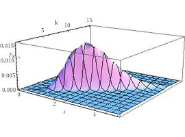
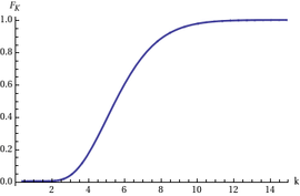
With a sample size and , you may find the joint p.d.f. of the Gamma parameters K and on the left. The marginal distribution of K is reported in the picture on the right.
Notes
- By default, capital letters (such as U, X) will denote random variables and small letters (u, x) their corresponding realizations.
References
- Fisher, M.A. (1935). "The fiducial argument in statistical inference". Annals of Eugenics. 6 (4): 391–398. doi:10.1111/j.1469-1809.1935.tb02120.x. hdl:2440/15222.CS1 maint: ref=harv (link)
- Fraser, D. A. S. (1966). "Structural probability and generalization". Biometrika. 53 (1/2): 1–9. doi:10.2307/2334048. JSTOR 2334048.CS1 maint: ref=harv (link)
- Apolloni, B; Malchiodi, D.; Gaito, S. (2006). Algorithmic Inference in Machine Learning. International Series on Advanced Intelligence. 5 (2nd ed.). Adelaide: Magill.
Advanced Knowledge International