Symmetry of second derivatives

In mathematics, the symmetry of second derivatives (also called the equality of mixed partials) refers to the possibility under certain conditions (see below) of interchanging the order of taking partial derivatives of a function

${\displaystyle f\left(x_{1},\,x_{2},\,\ldots ,\,x_{n}\right)}$

of n variables. If the partial derivative with respect to ${\displaystyle x_{i}}$ is denoted with a subscript ${\displaystyle i}$, then the symmetry is the assertion that the second-order partial derivatives ${\displaystyle f_{ij}}$ satisfy the identity

${\displaystyle f_{ij}=f_{ji}}$

so that they form an n × n symmetric matrix. This is sometimes known as Schwarz's theorem, Clairaut's theorem, or Young's theorem.[1][2]

In the context of partial differential equations it is called the Schwarz integrability condition.

Hessian matrix

This matrix of second-order partial derivatives of f is called the Hessian matrix of f. The entries in it off the main diagonal are the mixed derivatives; that is, successive partial derivatives with respect to different variables.

In most "real-life" circumstances the Hessian matrix is symmetric, although there are many functions that do not have this property. Mathematical analysis reveals that symmetry requires a hypothesis on f that goes further than simply stating the existence of the second derivatives at a particular point. The theorem of Schwarz gives a sufficient condition on f for this to occur.

Formal expressions of symmetry

In symbols, the symmetry may be expressed as:

${\displaystyle {\frac {\partial }{\partial x}}\left({\frac {\partial f}{\partial y}}\right)\ =\ {\frac {\partial }{\partial y}}\left({\frac {\partial f}{\partial x}}\right)\qquad {\text{or}}\qquad {\frac {\partial ^{2}\!f}{\partial x\,\partial y}}\ =\ {\frac {\partial ^{2}\!f}{\partial y\,\partial x}}.}$

Another notation is:

${\displaystyle \partial _{x}\partial _{y}f=\partial _{y}\partial _{x}f.}$

In terms of composition of the differential operator D_i which takes the partial derivative with respect to x_i:

${\displaystyle D_{i}\circ D_{j}=D_{j}\circ D_{i}}$.

From this relation it follows that the ring of differential operators with constant coefficients, generated by the D_i, is commutative; but this is only true as operators over a domain of sufficiently differentiable functions. It is easy to check the symmetry as applied to monomials, so that one can take polynomials in the x_i as a domain. In fact smooth functions are another valid domain.

Theorem of Schwarz

In mathematical analysis, Schwarz's theorem (or Clairaut's theorem on equality of mixed partials)[3] named after Alexis Clairaut and Hermann Schwarz, states that if ${\displaystyle \left(a_{1},\,\ldots ,\,a_{n}\right)\in \mathbb {R} ^{n}}$, ${\displaystyle \Omega \subseteq \mathbb {R} ^{n}}$, some neighborhood of ${\displaystyle \left(a_{1},\,\ldots ,\,a_{n}\right)}$ is contained in ${\displaystyle \Omega }$,

${\displaystyle f\colon \Omega \to \mathbb {R} }$

and ${\displaystyle f}$ has continuous second partial derivatives at the point in ${\displaystyle \left(a_{1},\,\ldots ,\,a_{n}\right)}$, then ${\displaystyle \forall i,j\in \{1,\,2,\,\ldots ,\,n\},}$

${\displaystyle {\frac {\partial ^{2}}{\partial x_{i}\,\partial x_{j}}}f\left(a_{1},\,\ldots ,\,a_{n}\right)={\frac {\partial ^{2}}{\partial x_{j}\,\partial x_{i}}}f\left(a_{1},\,\ldots ,\,a_{n}\right).}$

The partial derivatives of this function commute at that point. One easy way to establish this theorem (in the case where ${\displaystyle n=2}$, ${\displaystyle i=1}$, and ${\displaystyle j=2}$, which readily entails the result in general) is by applying Green's theorem to the gradient of ${\displaystyle f.}$

An elementary proof for functions on open subsets of the plane is as follows (by a simple reduction the general case for the theorem of Schwarz clearly reduces to the planar case).[4] Let ${\displaystyle f}$ be a differentiable function on an open rectangle containing ${\displaystyle (a,b)}$ and suppose that ${\displaystyle df}$ is continuous with ${\displaystyle \partial _{x}\partial _{y}f}$ and ${\displaystyle \partial _{y}\partial _{x}f}$ both continuous. Define

${\displaystyle {\begin{aligned}u\left(h,\,k\right)&=f\left(a+h,\,b+k\right)-f\left(a+h,\,b\right),\\v\left(h,\,k\right)&=f\left(a+h,\,b+k\right)-f\left(a,\,b+k\right),\\w\left(h,\,k\right)&=f\left(a+h,\,b+k\right)-f\left(a+h,\,b\right)-f\left(a,\,b+k\right)+f\left(a,\,b\right).\end{aligned}}}$

These functions are defined for ${\displaystyle \left|h\right|,\,\left|k\right|<\varepsilon }$, where ${\displaystyle \varepsilon >0}$ and ${\displaystyle \left[a-\varepsilon ,\,a+\varepsilon \right]\times \left[b-\varepsilon ,\,b+\varepsilon \right]\subset \Omega }$.

By the mean value theorem, intermediate values ${\displaystyle \theta ,\,\theta ^{\prime },\,\,\phi ,\,\,\phi ^{\prime }}$ can be found in ${\displaystyle (0,1)}$ with

${\displaystyle {\begin{aligned}w\left(h,\,k\right)&=u\left(h,\,k\right)-u\left(0,\,k\right)=h\,\partial _{x}u\left(\theta h,\,k\right)\\&=h\,\left[\partial _{x}f\left(a+\theta h,\,b+k\right)-\partial _{x}f\left(a+\theta h,\,b\right)\right]\\&=hk\,\partial _{y}\partial _{x}f\left(a+\theta h,\,b+\theta ^{\prime }k\right)\\w\left(h,\,k\right)&=v\left(h,\,k\right)-v\left(h,\,0\right)=k\,\partial _{y}v\left(h,\,\phi k\right)\\&=k\left[\partial _{y}f\left(a+h,\,b+\phi k\right)-\partial _{y}f\left(a,\,b+\phi k\right)\right]\\&=hk\,\partial _{x}\partial _{y}f\left(a+\phi ^{\prime }h,\,b+\phi k\right).\end{aligned}}}$

Since ${\displaystyle h,\,k\neq 0}$, the first equality below can be divided by ${\displaystyle hk}$:

${\displaystyle {\begin{aligned}hk\,\partial _{y}\partial _{x}f\left(a+\theta h,\,b+\theta ^{\prime }k\right)&=hk\,\partial _{x}\partial _{y}f\left(a+\phi ^{\prime }h,\,b+\phi k\right),\\\partial _{y}\partial _{x}f\left(a+\theta h,\,b+\theta ^{\prime }k\right)&=\partial _{x}\partial _{y}f\left(a+\phi ^{\prime }h,\,b+\phi k\right).\end{aligned}}}$

Letting ${\displaystyle h,\,k}$ tend to zero in the last equality, the continuity assumptions on ${\displaystyle \partial _{y}\partial _{x}f}$ and ${\displaystyle \partial _{x}\partial _{y}f}$ now imply that

${\displaystyle {\frac {\partial ^{2}}{\partial x\partial y}}f\left(a,\,b\right)={\frac {\partial ^{2}}{\partial y\partial x}}f\left(a,\,b\right).}$

This account is a straightforward classical method found in many text books, for example in Burkill, Apostol and Rudin.[5][6]

Although the derivation above is elementary, the approach can also be viewed from a more conceptual perspective so that the result becomes more apparent.[7][8][9][10][11] Indeed the difference operators ${\displaystyle \Delta _{x}^{t},\,\,\Delta _{y}^{t}}$ commute and ${\displaystyle \Delta _{x}^{t}f,\,\,\Delta _{y}^{t}f}$ tend to ${\displaystyle \partial _{x}f,\,\,\partial _{y}f}$ as ${\displaystyle t}$ tends to 0, with a similar statement for second order operators.[12] Here, for ${\displaystyle z}$ a vector in the plane and ${\displaystyle u}$ a directional vector, the difference operator is defined by

${\displaystyle \Delta _{u}^{t}f(z)={f(z+tu)-f(z) \over t}.}$

By the fundamental theorem of calculus for ${\displaystyle C^{1}}$ functions ${\displaystyle f}$ on an open interval ${\displaystyle I}$ with ${\displaystyle (a.b)\subset I}$

${\displaystyle \int _{a}^{b}f^{\prime }(x)\,dx=f(b)-f(a).}$

Hence

${\displaystyle |f(b)-f(a)|\leq (b-a)\,\sup _{c\in (a,b)}|f^{\prime }(c)|}$.

This is a generalized version of the mean value theorem. Recall that the elementary discussion on maxima or minima for real-valued functions implies that if ${\displaystyle f}$ is continuous on ${\displaystyle [a,b]}$ and differentiable on ${\displaystyle (a,b)}$, then there is a point ${\displaystyle c}$ in ${\displaystyle (a,b)}$ such that

${\displaystyle {f(b)-f(a) \over b-a}=f^{\prime }(c).}$

For vector-valued functions with ${\displaystyle V}$ a finite-dimensional normed space, there is no analogue of the equality above, indeed it fails. But since ${\displaystyle \inf f^{\prime }\leq f^{\prime }(c)\leq \sup f^{\prime }}$, the inequality above is a useful substitute. Moreover, using the pairing of the dual of ${\displaystyle V}$ with its dual norm, yields the following equality:

${\displaystyle \|f(b)-f(a)\|\leq (b-a)\,\sup _{c\in (a,b)}\|f^{\prime }(c)\|}$.

These versions of the mean valued theorem are discussed in Rudin, Hörmander and elsewhere.[13][14]

For ${\displaystyle f}$ a ${\displaystyle C^{2}}$ function on an open set in the plane, define ${\displaystyle D_{1}=\partial _{x}}$ and ${\displaystyle D_{2}=\partial _{y}}$. Furthermore for ${\displaystyle t\neq 0}$ set

${\displaystyle \Delta _{1}^{t}f(x,y)=[f(x+t,y)-f(x,y)]/t,\,\,\,\,\,\,\Delta _{2}^{t}f(x,y)=[f(x,y+t)-f(x,y)]/t}$.

Then for ${\displaystyle (x_{0},y_{0})}$ in the open set, the generalized mean value theorem can be applied twice:

${\displaystyle \left|\Delta _{1}^{t}\Delta _{2}^{t}f(x_{0},y_{0})-D_{1}D_{2}f(x_{0},y_{0})\right|\leq \sup _{0\leq s\leq 1}\left|\Delta _{1}^{t}D_{2}f(x_{0},y_{0}+ts)-D_{1}D_{2}f(x_{0},y_{0})\right|\leq \sup _{0\leq r,s\leq 1}\left|D_{1}D_{2}f(x_{0}+tr,y_{0}+ts)-D_{1}D_{2}f(x_{0},y_{0})\right|.}$

Thus ${\displaystyle \Delta _{1}^{t}\Delta _{2}^{t}f(x_{0},y_{0})}$ tends to ${\displaystyle D_{1}D_{2}f(x_{0},y_{0})}$ as ${\displaystyle t}$ tends to 0. The same argument shows that ${\displaystyle \Delta _{2}^{t}\Delta _{1}^{t}f(x_{0},y_{0})}$ tends to ${\displaystyle D_{2}D_{1}f(x_{0},y_{0})}$. Hence, since the difference operators commute, so do the partial differential operators ${\displaystyle D_{1}}$ and ${\displaystyle D_{2}}$, as claimed.[15][16][17][18][19]

Remark. By two applications of the classical mean value theorem,

${\displaystyle \Delta _{1}^{t}\Delta _{2}^{t}f(x_{0},y_{0})=D_{1}D_{2}f(x_{0}+t\theta ,y_{0}+t\theta ^{\prime })}$

for some ${\displaystyle \theta }$ and ${\displaystyle \theta ^{\prime }}$ in ${\displaystyle (0,1)}$. Thus the first elementary proof can be reinterpreted using difference operators. Conversely, instead of using the generalized mean value theorem in the second proof, the classical mean valued theorem could be used. Since it was first established in 1883, Camille Jordan's 19th-century proof of symmetry of second mixed derivatives has been described as "perfect".[20][21]

Theorems of Fubini and Clairaut

Let ${\displaystyle I}$ and ${\displaystyle J}$ be closed intervals in the real line and let ${\displaystyle F(x,y)}$ be a continuous function on ${\displaystyle I\times J}$. Thus ${\displaystyle F}$ is uniformly continuous on ${\displaystyle I\times J}$. One of the main steps in establishing Fubini's theorem is to show that for any such ${\displaystyle F}$

${\displaystyle \sup _{y}\left|\int _{I}F(x,y)\,dx\right|\leq |I|\cdot \|F\|_{\infty },\,\,\,\sup _{x}\left|\int _{J}F(x,y)\,dy\right|\leq |J|\cdot \|F\|_{\infty }.}$

The first task is to prove Dieudonné's theorem: that any continuous function ${\displaystyle F(x,y)}$ on ${\displaystyle I\times J}$ can be approximated uniformly by a finite sum ${\displaystyle \sum _{i}g_{i}(x)h_{i}(y)}$. Approximations of this kind were known to be consequences of the Stone-Weierstrass theorem established in the 1940s. Earlier Jean Dieudonné succeeded in proving these directly in 1937 using simpler methods.[22][23][24]

Given ${\displaystyle n>0}$, there are triangular functions ${\displaystyle 0\leq \varphi _{i}\leq 1}$ with ${\displaystyle 0\leq i\leq n}$ such that

${\displaystyle \sum _{i}\varphi _{i}=1,}$

and each ${\displaystyle \varphi _{i}}$ is supported in intervals ${\displaystyle I_{i}}$ of length less than ${\displaystyle 2|I|/n}$. The family ${\displaystyle (\varphi _{i})}$ is thus an example of a continuous "partition of unity": these were first defined by Dieudonné for solving exactly these kinds of problems.[25] By uniform continuity of ${\displaystyle F}$, given ${\displaystyle \varepsilon >0}$, there is a constant ${\displaystyle \delta >0}$ such that ${\displaystyle |F(a,y)-F(b,y)|\leq \varepsilon }$ whenever ${\displaystyle |a-b|\leq \delta }$ and ${\displaystyle y\in J}$. Here ${\displaystyle n}$ can chosen sufficiently large that every interval ${\displaystyle I_{i}}$ is less than ${\displaystyle \delta }$. Choose ${\displaystyle a_{i}\in I_{i}}$ for each ${\displaystyle 0\leq i\leq n}$ and set

${\displaystyle g_{i}(x)=\varphi _{i}(x),\,\,\,h_{i}(y)=F(a_{i},y),\,\,\,\,F_{n}(x,y)=\sum _{i}g_{i}(x)h_{i}(y).}$

Then for all ${\displaystyle x,y}$

${\displaystyle |F_{n}(x,y)-F(x,y)|\leq \varepsilon ,}$

so that ${\displaystyle F_{n}}$ tends to ${\displaystyle F}$ uniformly.

In fact to check the estimate above, note that

${\displaystyle |F_{n}(x,y)-F(x,y)|\leq \sum _{i}\varphi _{i}(x)|F(a_{i},y)-F(x,y)|\leq \sum _{i}\varphi _{i}(x)\varepsilon =\varepsilon ,}$

observing that ${\displaystyle \varphi _{i}}$ vanishes off ${\displaystyle I_{i}}$.

Fubini's theorem can now be established by formally defining iterated Riemann integrals for simple functions ${\displaystyle \sum _{i}g_{i}(x)h_{i}(y)}$ and then passing to the limit by continuity. This follows the framework developed for the Daniell integral by Loomis (1953), but in a very much simplified setting. Real-valued functions will be used here, but—as with the Riemann integration in one variable—the passage to complex-valued functions is routine.

Let ${\displaystyle {\cal {I}}}$ be denote Riemann integration on ${\displaystyle x}$ for intervals. Then for ${\displaystyle g}$ in ${\displaystyle C_{\rm {R}}(I)}$,

${\displaystyle |{\cal {I}}(g)|\leq |I|\cdot \|g\|_{\infty }.}$

For, if ${\displaystyle g}$ is real, then ${\displaystyle -\|g\|_{\infty }\leq g\leq \|g\|_{\infty }}$. The form ${\displaystyle {\cal {I}}}$ is positive since ${\displaystyle {\cal {I}}(1)=|I|}$ and, if ${\displaystyle g\geq c>0}$ then ${\displaystyle {\cal {I}}(g)\geq c\cdot |I|}$. Thus ${\displaystyle {\cal {I}}(g)>0}$ if ${\displaystyle g>0}$.

Similarly for integration ${\displaystyle {\cal {J}}}$ on ${\displaystyle x}$ and ${\displaystyle h}$ in ${\displaystyle C_{\rm {R}}(J)}$,

${\displaystyle |{\cal {J}}(h)|\leq |J|\cdot \|h\|_{\infty },}$

with ${\displaystyle {\cal {J}}(h)>0}$ if ${\displaystyle h>0}$.

For functions given by finite sums ${\displaystyle K=\sum _{i}g_{i}(x)h_{i}(y)}$ in ${\displaystyle C_{\rm {R}}(I\times J)}$

${\displaystyle \left|({\cal {I}}{\cal {J}})(K)\right|=\left|\sum _{i}{\cal {I}}(g_{i})\,{\cal {J}}(h_{i})\right|\leq |I|\cdot |J|\cdot \|K\|_{\infty }.}$

It will be established that ${\displaystyle {\cal {I}}{\cal {J}}={\cal {J}}{\cal {I}}}$ also defines a positive form; and that if ${\displaystyle F>0}$, then ${\displaystyle {\cal {I}}{\cal {J}}(F)={\cal {J}}{\cal {I}}(F)>0}$.

These inequalities can be extended to ${\displaystyle F}$ in ${\displaystyle C_{\rm {R}}(I\times J)}$ by approximately such finite sums ${\displaystyle K}$ uniformly. Indeed if ${\displaystyle \|F-K\|_{\infty }<\varepsilon }$,

${\displaystyle |{\cal {J}}(F-K)|<|J|\cdot \varepsilon .}$

Thus ${\displaystyle K_{n}}$ tends uniformly to ${\displaystyle F}$, ${\displaystyle {\cal {{J}(K_{n})}}}$ tends to uniformly to ${\displaystyle {\cal {{J}(F)}}}$, which must therefore be in ${\displaystyle C_{\rm {R}}(I)}$.

Finally, on integrating over ${\displaystyle x}$, it follows that ${\displaystyle {\cal {I}}{\cal {J}}(K_{n})}$ tends to ${\displaystyle {\cal {I}}{\cal {J}}(F)}$ with ${\displaystyle |{\cal {I}}{\cal {J}}(F)|\leq |I|\cdot |J|\cdot \|F\|_{\infty }}$. Similarly, taking the limits over ${\displaystyle x}$ and then ${\displaystyle y}$, the integrals ${\displaystyle {\cal {I}}{\cal {J}}(K_{n})}$ tend to ${\displaystyle {\cal {I}}{\cal {J}}(F)}$. But for ${\displaystyle K_{n}}$, it was seen that integrating in the different order gives the same answer ${\displaystyle \sum _{i}{\cal {I}}(g_{i}){\cal {J}}(h_{i})}$.

Summarising, for ${\displaystyle F}$ in ${\displaystyle C_{\rm {R}}(I\times J)}$, the following equality for iterated integral holds:

${\displaystyle {\cal {I}}{\cal {J}}(F)={\cal {J}}{\cal {I}}(F).}$

This is Fubini's theorem in the special case of ${\displaystyle I\times J}$.[26][27]

To prove Clairaut's theorem,[28][29][30] let ${\displaystyle f}$ be differentiable on the open set ${\displaystyle U}$ in the plane with both ${\displaystyle f_{xy}}$ and ${\displaystyle f_{yx}}$ continuous. Taking a rectangle ${\displaystyle [a,b]\times [c,d]}$ the integral can be computed using the fundamental theorem of calculus

${\displaystyle {\cal {J}}{\cal {I}}(f_{xy})=f(a,c)+f(b,d)-f(b,d)-f(a,d).}$

Similarly

${\displaystyle {\cal {I}}{\cal {J}}(f_{yx})=f(a,c)+f(b,d)-f(b,d)-f(a,d).}$

The hypotheses of continuity and Fubini's theorem implies that ${\displaystyle {\cal {J}}{\cal {I}}(f_{xy})={\cal {I}}{\cal {J}}(f_{xy})}$ for any rectangle. Since ${\displaystyle {\cal {I}}{\cal {J}}}$ is a positive form, if ${\displaystyle f_{xy}-f_{yx}}$ or its negative became strictly positive on the rectangle, this would give a contradiction.

Sufficiency of twice-differentiability

A weaker condition than the continuity of second partial derivatives (which is implied by the latter) which suffices to ensure symmetry is that all partial derivatives are themselves differentiable.[31] Another strengthening of the theorem, in which existence of the permuted mixed partial is asserted, was provided by Peano in a short 1890 note on Mathesis:

If ${\displaystyle f:E\to \mathbb {R} }$ is defined on an open set ${\displaystyle E\subset \mathbb {R} ^{2}}$; ${\displaystyle \partial _{1}f(x,\,y)}$ and ${\displaystyle \partial _{2,1}f(x,\,y)}$ exist everywhere on ${\displaystyle E}$; ${\displaystyle \partial _{2,1}f}$ is continuous at ${\displaystyle \left(x_{0},\,y_{0}\right)\in E}$, and if ${\displaystyle \partial _{2}f(x,\,y_{0})}$ exists in a neighborhood of ${\displaystyle x=x_{0}}$, then ${\displaystyle \partial _{1,2}f}$ exists at ${\displaystyle \left(x_{0},\,y_{0}\right)}$ and ${\displaystyle \partial _{1,2}f\left(x_{0},\,y_{0}\right)=\partial _{2,1}f\left(x_{0},\,y_{0}\right)}$.[32]

History

The result of the equality of the mixed partial derivatives under certain conditions has a long history. Nicolaus I Bernoulli implicitly assumed the result as early as 1721, but Euler was the first to provide a proof. Other proofs followed by Clairaut (1740), Lagrange (1797), Cauchy (1823) and many others in the 19th century. None of these proofs were without fault however (for example, Clairaut assumed all definite integrals could be differentiated under the integral sign). In 1867 Ernst Leonard Lindelöf published a paper[33] criticizing in detail all the proofs he was familiar with. Finally, six years later Hermann Schwarz (1873) gave the first satisfactory proof. This was followed by successive refinements that relaxed the hypotheses in Schwarz's theorem in various ways, among others by Dini, Jordan, Peano, E. W. Hobson, W. H. Young. For a good historical account, see Higgins (1940).[21].

Most advanced calculus texts contain sufficient conditions and proof for the equality of second mixed partial derivatives. Hence this is something that should interest those involved in teaching and learning that part of analysis. The topic can be separated into be divided into two distinct line of attack. The first came in 1867 when, following many announcements of incomplete proofs, the Finnish mathematician Lindelöf found a counter-example. The second in 1873 was the success by the German analyst H. A. Schwarz in discovering a first rigorous proof of sufficient conditions.

In 1898 Moritz Cantor outlined the historical status of second mixed derivatives before 1800. In 1740 Leonard Euler was the first to publish a proposed proof. However, already in 1721, the works of Nicolas Bernoulli had tacitly assumed the property without any formal proof. At the same time as Euler, Clairaut proposed a proof, unchallenged for most of the century. Then successively Lagrange (1797), Cauchy (1823), P. Blanchet (1841), Duhamel (1856), Sturm (1857), Schlömilch (1862), and Bertrand (1864) published incomplete proofs. All of the proposed proofs had been criticized, particularly when subtle points on limiting procedures arose. It was as a result of a detailed study of the deficiencies that Lindelöf could explicitly exhibit a counter-example, thus ending the stage of "primitive" investigations.

Six years after Lindelöf, Schwarz published the first satisfactory proof, thus starting the next stage of investigations. Mathematicians tried to relax some of the assumptions of Schwarz. After an unsuccessful attempt by Thomae in 1875, the Italian mathematician Dini made an improved on Schwarz by introducing the more general "Dini-Schwarz conditions". Following another fruitless effort by Harnack in 1881, Jordan in 1882 was able to make headway. Assuming less than Dini, he published in 1883 the proof that can now be found in most text books. Along with this popular account, there are other versions by Laurent (1885), Peano (1889 and 1893), J. Edwards (1892), P. Haag (1893), J. K. Whittemore (1898), Vivanti (1899), and Pierpont (1905). Some of these expositions were perfect, some not, but essentially apart from changing some points of view in a minor way, Jordan's proof was adopted.

Further advances were made by E. W. Hobson in 1907 when he introduced successive differentiation, further relaxing the Dini-Schwarz conditions. Later in 1909, W. H. Young independently found less restrictions than the Dini-Schwarz conditions. Just at that time Young published a theorem which he referred to as him as "the fundamental theorem of the theory of differentials of two variables" stating that "if ${\displaystyle u_{x}}$ and ${\displaystyle u_{y}}$ each have differentials of the first order, the function ${\displaystyle u}$ possesses a differential of the second order." In his proof, he showed that in those particular circumstances the function had equal mixed second derivatives. Finally, in 1918, Carathéodory gave an original and unique contribution in this context using Lebesgue integration.[21]

Distribution theory formulation

The theory of distributions (generalized functions) eliminates analytic problems with the symmetry. The derivative of an integrable function can always be defined as a distribution, and symmetry of mixed partial derivatives always holds as an equality of distributions. The use of formal integration by parts to define differentiation of distributions puts the symmetry question back onto the test functions, which are smooth and certainly satisfy this symmetry. In more detail (where f is a distribution, written as an operator on test functions, and φ is a test function),

${\displaystyle \left(D_{1}D_{2}f\right)[\phi ]=-\left(D_{2}f\right)\left[D_{1}\phi \right]=f\left[D_{2}D_{1}\phi \right]=f\left[D_{1}D_{2}\phi \right]=-\left(D_{1}f\right)\left[D_{2}\phi \right]=\left(D_{2}D_{1}f\right)[\phi ].}$

Another approach, which defines the Fourier transform of a function, is to note that on such transforms partial derivatives become multiplication operators that commute much more obviously.[12]

Requirement of continuity

The symmetry may be broken if the function fails to have differentiable partial derivatives, which is possible if Clairaut's theorem is not satisfied (the second partial derivatives are not continuous).

The function f(x, y), as shown in equation (1), does not have symmetric second derivatives at its origin.

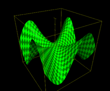
An example of non-symmetry is the function (due to Peano)[34][35]

${\displaystyle f(x,\,y)={\begin{cases}{\frac {xy\left(x^{2}-y^{2}\right)}{x^{2}+y^{2}}}&{\mbox{ for }}(x,\,y)\neq (0,\,0)\\0&{\mbox{ for }}(x,\,y)=(0,\,0).\end{cases}}}$

(1)

This can be visualized by the polar form ${\displaystyle f(r\cos(\theta ),r\sin(\theta ))=r^{2}\sin(4\theta )}$; it is everywhere continuous, but its derivatives at (0, 0) cannot be computed algebraically. Rather, the limit of difference quotients shows that ${\displaystyle \left.\partial _{x}f\right|_{(0,0)}=\left.\partial _{y}f\right|_{(0,0)}=0}$, so the graph z = f(x, y) has a horizontal tangent plane at (0, 0), and the partial derivatives ${\displaystyle \partial _{x}f,\partial _{y}f}$ exist and are everywhere continuous. However, the second partial derivatives are not continuous at (0, 0), and the symmetry fails. In fact, along the x-axis the y-derivative is ${\displaystyle \left.\partial _{y}f\right|_{(x,0)}=x}$, and so:

${\displaystyle \left.\partial _{x}\partial _{y}f\right|_{(0,0)}=\lim _{\varepsilon \rightarrow 0}{\frac {\left.\partial _{y}f\right|_{(\varepsilon ,0)}-\left.\partial _{y}f\right|_{(0,0)}}{\varepsilon }}=1.}$

In contrast, along the y-axis the x-derivative ${\displaystyle \left.\partial _{x}f\right|_{(0,y)}=-y}$, and so ${\displaystyle \left.\partial _{y}\partial _{x}f\right|_{(0,0)}=-1}$. That is, ${\displaystyle \partial _{xy}f\neq \partial _{yx}f}$ at (0, 0), although the mixed partial derivatives do exist, and at every other point the symmetry does hold.

The above function, written in a cylindrical coordinate system, can be expressed as

${\displaystyle f(r,\,\theta )={\frac {r^{2}\sin {4\theta }}{4}},}$

showing that the function oscillates four times when traveling once around an arbitrarily small loop containing the origin. Intuitively, therefore, the local behavior of the function at ${\displaystyle (0,\,0)}$ cannot be described as a quadratic form, and the Hessian matrix thus fails to be symmetric.

In general, the interchange of limiting operations need not commute. Given two variables near (0, 0) and two limiting processes on

${\displaystyle f(h,\,k)-f(h,\,0)-f(0,\,k)+f(0,\,0)}$

corresponding to making h → 0 first, and to making k → 0 first. It can matter, looking at the first-order terms, which is applied first. This leads to the construction of pathological examples in which second derivatives are non-symmetric. This kind of example belongs to the theory of real analysis where the pointwise value of functions matters. When viewed as a distribution the second partial derivative's values can be changed at an arbitrary set of points as long as this has Lebesgue measure 0. Since in the example the Hessian is symmetric everywhere except (0, 0), there is no contradiction with the fact that the Hessian, viewed as a Schwartz distribution, is symmetric.

In Lie theory

Consider the first-order differential operators D_i to be infinitesimal operators on Euclidean space. That is, D_i in a sense generates the one-parameter group of translations parallel to the x_i-axis. These groups commute with each other, and therefore the infinitesimal generators do also; the Lie bracket

[D_i, D_j] = 0

is this property's reflection. In other words, the Lie derivative of one coordinate with respect to another is zero.

Application to differential forms

The Clairaut-Schwarz theorem is the key fact needed to prove that for every ${\displaystyle C^{\infty }}$ (or at least twice differentiable) differential form ${\displaystyle \omega \in \Omega ^{k}(M)}$, the second exterior derivative vanishes: ${\displaystyle d^{2}\omega$ :=d(d\omega )=0} . This implies that every differentiable exact form (i.e., a form ${\displaystyle \alpha }$ such that ${\displaystyle \alpha =d\omega }$ for some form ${\displaystyle \omega }$) is closed (i.e., ${\displaystyle d\alpha =0}$), since ${\displaystyle d\alpha =d(d\omega )=0}$.[36]

In the middle of the 18th century, the theory of differential forms first studied in the simplest case of 1-forms in the plane, i.e. ${\displaystyle Adx+Bdy}$, where ${\displaystyle A}$ and ${\displaystyle B}$ are functions in the plane. The study of 1-forms and the differentials of functions began with Clairaut's papers in 1739 and 1740. At that stage his investigations were interpreted as ways of solving ordinary differential equations. Formally Clairaut showed that a 1-form ${\displaystyle \omega =Adx+Bdy}$ on an open rectangle is closed, i.e. ${\displaystyle d\omega =0}$, if and only ${\displaystyle \omega }$ has the form ${\displaystyle df}$ for some function ${\displaystyle f}$ in the disk. The solution for ${\displaystyle f}$ can be written by Cauchy's integral formula

${\displaystyle f(x,y)=\int _{x_{0}}^{x}A(x,y)\,dx+\int _{y_{0}}^{y}B(x,y)\,dy;}$

while if ${\displaystyle \omega =df}$, the closed property ${\displaystyle d\omega =0}$ is the identity ${\displaystyle \partial _{x}\partial _{y}f=\partial _{y}\partial _{x}f}$. (In modern language this is one version of the Poincaré lemma.)[37]

Notes

1. "Young's Theorem" (PDF). Archived from the original (PDF) on May 18, 2006. Retrieved 2015-01-02.
2. Allen, R. G. D. (1964). Mathematical Analysis for Economists. New York: St. Martin's Press. pp. 300–305.
3. James, R. C. (1966). Advanced Calculus. Belmont, CA: Wadsworth.
4. Burkill 1962, pp. 154-155
5. Apostol 1965 harvnb error: no target: CITEREFApostol1965 (help)
6. Rudin 1976 harvnb error: multiple targets (2×): CITEREFRudin1976 (help)
7. Hörmander 2015, pp. 7,11. This condensed account is possibly the shortest.
8. Dieudonné 1960, pp. 179-180
9. Godement 1998b, pp. 287-289
10. Lang 1969, pp. 108-111
11. Cartan 1971, pp. 64-67
12. These can also be rephrased in terms of the action of operators on Schwartz functions on the plane. Under Fourier transform, the difference and differential operators are just multiplication operators. See Hörmander (2015), Chapter VII.
13. Hörmander 2015, p. 6
14. Rudin 1976 harvnb error: multiple targets (2×): CITEREFRudin1976 (help)
15. Hörmander 2015, p. 11
16. Dieudonné 1960
17. Godement 1998a
18. Lang 1969
19. Cartan 1971
20. Jordan 1893, pp. 118-119
21. Higgins, Thomas James (1940). "A note on the history of mixed partial derivatives". Scripta Mathematica. 7: 59–62. Retrieved 19 April 2017.
22. Dieudonné 1937
23. Nachbin 1965, pp. 57-58
24. Dieudonné 1976, pp. 20-22, 220-221
25. Hörmander 2015, pp. 25-32
26. Loomis 1953, p. 42
27. Dieudonné 1976, pp. 219-222
28. Spivak 1965, p. 61
29. McGrath 2014
30. See Donald E. Marshall's note
31. Hubbard, John; Hubbard, Barbara. Vector Calculus, Linear Algebra and Differential Forms (5th ed.). Matrix Editions. pp. 732–733.
32. Rudin, Walter (1976). Principles of Mathematical Analysis. New York: McGraw-Hill. pp. 235–236. ISBN 0-07-054235-X.
33. Lindelöf, Ernst Leonard (1867). "Remarques sur les différentes manières d'établir la formule ${\displaystyle {\frac {d^{2}z}{dxdy}}={\frac {d^{2}z}{dydx}}}$". Acta Societatis Scientiarum Fennicae. 8, part 1: 205–213.
34. Hobson 1921, pp. 403-404
35. Apostol 1974, pp. 358-359
36. Tu, Loring W. (2010). An Introduction to Manifolds (2nd ed.). New York: Springer. ISBN 978-1-4419-7399-3.
37. Katz 1981

References

• Aksoy, A.; Martelli, M. (2002), "Mixed Partial Derivatives and Fubini's Theorem", College Mathematics Journal of MAA, 33: 126–130
• Apostol, Tom M. (1974), Mathematical Analysis, Addison-Wesley, ISBN 9780201002881
• Burkill, J. C. (1962), A First Course in Mathematical Analysis, Cambridge University Press, ISBN 9780521294683 (reprinted 1978)
• Cartan, Henri (1971), Calcul Differentiel (in French), Hermann, ISBN 9780395120330
• Clairaut, A.C. (1739), "Recherches générales sur le calcul intégral", Memoires de l'Académie Royale des Sciences: 425–436
• Clairaut, A. C. (1740), "Sur l'integration ou la construction des equations différentielles du premier ordre", Memoires de l'Académie Royale des Sciences, 2: 293–323
• Dieudonné, J. (1937), "Sur les fonctions continues numérique définies dans une produit de deux espaces compacts", Comptes Rendus Acad. Sci. Paris, 205: 593–595
• Dieudonné, J. (1960), Foundations of Modern Analysis, Pure and Applied Mathematics, 10, Academic Press, ISBN 9780122155505
• Dieudonné, J. (1976), Treatise on analysis. Vol. II., Pure and Applied Mathematics, 10-II, translated by I. G. Macdonald, Academic Press, ISBN 9780122155024
• Gilkey, Peter; Park, JeongHyeong; Vázquez-Lorenzo, Ramón (2015), Aspects of differential geometry I, Synthesis Lectures on Mathematics and Statistics, 15, Morgan & Claypool, ISBN 9781627056632
• Godement, Roger (1998a), Analyse mathématique I (PDF), Springer
• Godement, Roger (1998b), Analyse mathématique II (PDF), Springer
• Hobson, E. W. (1921), The theory of functions of a real variable and the theory of Fourier's series. Vol. I., Cambridge University Press
• Hörmander, Lars (2015), The Analysis of Linear Partial Differential Operators I: Distribution Theory and Fourier Analysis, Classics in Mathematics (2nd ed.), Springer, ISBN 9783642614972
• Jordan, Camille (1893), Cours d'analyse de l'École polytechnique. Tome I. Calcul différentiel (Les Grands Classiques Gauthier-Villars), Éditions Jacques Gaba]
• Katz, Victor J. (1981), "The history of differential forms from Clairaut to Poincaré", Historia Mathematica, 8: 161–188
• Lang, Serge (1969), Real Analysis, Addison-Wesley, ISBN 0201041790
• Lindelöf, E. L. (1867), "Remarques sur les différentes manières d'établir la formule d² z/dx dy = d² z/dy dx", Acta Societatis Scientiarum Fennicae, 8: 205–213
• Loomis, Lynn H. (1953), An introduction to abstract harmonic analysis, D. Van Nostrand
• Marshall, Donald E., Informal note on Theorems of Fubini and Clairaut (PDF), University of Washington
• McGrath, Peter J. (2014), "Another proof of Clairaut's theorem", Amer. Math. Monthly, 121: 165–166
• Nachbin, Leopoldo (1965), Elements of approximation theory, Notas de Matemática, 33, Rio de Janeiro: Fascículo publicado pelo Instituto de Matemática Pura e Aplicada do Conselho Nacional de Pesquisas
• Rudin, Walter (1976), Principles of Mathematical Analysis, International Series in Pure & Applied Mathematics, McGraw-Hill, ISBN 007054235X
• Schwarz, H. A. (1873), "Communication", Archives des Sciences Physiques et Naturelles, 48: 38–44
• Spivak, Michael (1965), Calculus on manifolds. A modern approach to classical theorems of advanced calculus, W. A. Benjamin
• Tao, Terence (2006), Analysis II (PDF), Texts and Readings in Mathematics, 38, Hindustan Book Agency, ISBN 8185931631

Further reading

• "Partial derivative", Encyclopedia of Mathematics, EMS Press, 2001 [1994]