Summed-area table

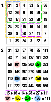
A summed-area table is a data structure and algorithm for quickly and efficiently generating the sum of values in a rectangular subset of a grid. In the image processing domain, it is also known as an integral image. It was introduced to computer graphics in 1984 by Frank Crow for use with mipmaps. In computer vision it was popularized by Lewis[1] and then given the name "integral image" and prominently used within the Viola–Jones object detection framework in 2001. Historically, this principle is very well known in the study of multi-dimensional probability distribution functions, namely in computing 2D (or ND) probabilities (area under the probability distribution) from the respective cumulative distribution functions.[2]

Using a summed-area table (2.) of an order-6 magic square (1.) to sum up a subrectangle of its values; each coloured spot highlights the sum inside the rectangle of that colour.

The algorithm

As the name suggests, the value at any point (x, y) in the summed-area table is the sum of all the pixels above and to the left of (x, y), inclusive:[3][4]

${\displaystyle I(x,y)=\sum _{\begin{smallmatrix}x'\leq x\\y'\leq y\end{smallmatrix}}i(x',y')}$

where ${\displaystyle i(x,y)}$ is the value of the pixel at (x,y).

The summed-area table can be computed efficiently in a single pass over the image, as the value in the summed-area table at (x, y) is just:[5]

${\displaystyle I(x,y)=i(x,y)+I(x,y-1)+I(x-1,y)-I(x-1,y-1)\,}$ (Noted that the summed matrix is calculated from top left corner)

A description of computing a sum in the summed-area table data structure/algorithm

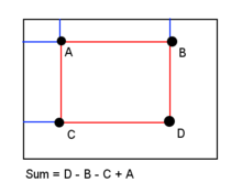
Once the summed-area table has been computed, evaluating the sum of intensities over any rectangular area requires exactly four array references regardless of the area size. That is, the notation in the figure at right, having A=(x₀, y₀), B=(x₁, y₀), C=(x₀, y₁) and D=(x₁, y₁), the sum of i(x,y) over the rectangle spanned by A, B,C and D is:

${\displaystyle \sum _{\begin{smallmatrix}x_{0}<x\leq x_{1}\\y_{0}<y\leq y_{1}\end{smallmatrix}}i(x,y)=I(D)+I(A)-I(B)-I(C)}$

Extensions

This method is naturally extended to continuous domains.[2]

The method can be also extended to high-dimensional images.[6] If the corners of the rectangle are ${\displaystyle x^{p}}$ with ${\displaystyle p}$ in ${\displaystyle \{0,1\}^{d}}$, then the sum of image values contained in the rectangle are computed with the formula

${\displaystyle \sum _{p\in \{0,1\}^{d}}(-1)^{d-\|p\|_{1}}I(x^{p})\,}$

where ${\displaystyle I(x)}$ is the integral image at ${\displaystyle x}$ and ${\displaystyle d}$ the image dimension. The notation ${\displaystyle x^{p}}$ correspond in the example to ${\displaystyle d=2}$, ${\displaystyle A=x^{(0,0)}}$, ${\displaystyle B=x^{(1,0)}}$, ${\displaystyle C=x^{(1,1)}}$ and ${\displaystyle D=x^{(0,1)}}$. In neuroimaging, for example, the images have dimension ${\displaystyle d=3}$ or ${\displaystyle d=4}$, when using voxels or voxels with a time-stamp.

This method has been extended to high-order integral image as in the work of Phan et al.[7] who provided two, three, or four integral images for quickly and efficiently calculating the standard deviation (variance), skewness, and kurtosis of local block in the image. This is detailed below:

To compute variance or standard deviation of a block, we need two integral images:

${\displaystyle I(x,y)=\sum _{\begin{smallmatrix}x'\leq x\\y'\leq y\end{smallmatrix}}i(x',y')}$

${\displaystyle I^{2}(x,y)=\sum _{\begin{smallmatrix}x'\leq x\\y'\leq y\end{smallmatrix}}i^{2}(x',y')}$

The variance is given by:

${\displaystyle \operatorname {Var} (X)={\frac {1}{n}}\sum _{i=1}^{n}(x_{i}-\mu )^{2}.}$

Let ${\displaystyle S_{1}}$ and ${\displaystyle S_{2}}$ denote the summations of block ${\displaystyle ABCD}$ of ${\displaystyle I}$ and ${\displaystyle I^{2}}$, respectively. ${\displaystyle S_{1}}$ and ${\displaystyle S_{2}}$ are computed quickly by integral image. Now, we manipulate the variance equation as:

${\displaystyle \operatorname {Var} (X)={\frac {1}{n}}\sum _{i=1}^{n}(x_{i}^{2}-2\cdot \mu \cdot x_{i}+\mu ^{2})={\frac {1}{n}}(\sum _{i=1}^{n}(x_{i})^{2}-2\cdot \sum _{i=1}^{n}(\mu \cdot x_{i})+\sum _{i=1}^{n}(\mu ^{2}))={\frac {1}{n}}(\sum _{i=1}^{n}(x_{i})^{2}-2\cdot \sum _{i=1}^{n}(\mu \cdot x_{i})+n\cdot (\mu ^{2}))}$

${\displaystyle ={\frac {1}{n}}(\sum _{i=1}^{n}(x_{i})^{2}-2\cdot \mu \cdot \sum _{i=1}^{n}(x_{i})+n\cdot (\mu ^{2}))={\frac {1}{n}}(S_{2}-2\cdot S_{1}/n\cdot S_{1}+n\cdot ((S_{1}/n)^{2}))={\frac {1}{n}}(S_{2}-(S_{1})^{2}/n)}$

Where ${\displaystyle \mu =S_{1}/n}$ and ${\displaystyle S_{2}=\sum _{i=1}^{n}(x_{i}^{2})}$.

Similar to the estimation of the mean (${\displaystyle \mu }$) and variance (${\displaystyle Var}$), which requires the integral images of the first and second power of the image respectively (i.e. ${\displaystyle I,I^{2}}$); manipulations similar to the ones mentioned above can be made to the third and fourth powers of the images (i.e. ${\displaystyle I^{3}(x,y),I^{4}(x,y)}$.) for obtaining the skewness and kurtosis.[7] But one important implementation detail that must be kept in mind for the above methods, as mentioned by F Shafait et al.[8] is that of integer overflow occurring for the higher order integral images in case 32-bit integers are used.

References

1. Lewis, J.P. (1995). Fast template matching. Proc. Vision Interface. pp. 120–123.
2. Finkelstein, Amir; neeratsharma (2010). "Double Integrals By Summing Values Of Cumulative Distribution Function". Wolfram Demonstration Project.
3. Crow, Franklin (1984). "Summed-area tables for texture mapping" (PDF). SIGGRAPH '84: Proceedings of the 11th annual conference on Computer graphics and interactive techniques. pp. 207–212.
4. Viola, Paul; Jones, Michael (2002). "Robust Real-time Object Detection" (PDF). International Journal of Computer Vision.
5. BADGERATI (2010-09-03). "Computer Vision – The Integral Image". computersciencesource.wordpress.com. Retrieved 2017-02-13.
6. Tapia, Ernesto (January 2011). "A note on the computation of high-dimensional integral images". Pattern Recognition Letters. 32 (2): 197–201. doi:10.1016/j.patrec.2010.10.007.
7. Phan, Thien; Sohoni, Sohum; Larson, Eric C.; Chandler, Damon M. (22 April 2012). Performance-analysis-based acceleration of image quality assessment (PDF). 2012 IEEE Southwest Symposium on Image Analysis and Interpretation. pp. 81–84. CiteSeerX 10.1.1.666.4791. doi:10.1109/SSIAI.2012.6202458. ISBN 978-1-4673-1830-3.
8. Shafait, Faisal; Keysers, Daniel; M. Breuel, Thomas (January 2008). "Efficient implementation of local adaptive thresholding techniques using integral images" (PDF). Electronic Imaging. Document Recognition and Retrieval XV. 6815: 681510–681510–6. CiteSeerX 10.1.1.109.2748. doi:10.1117/12.767755.

External links

• Summed table implementation in object detection

Lecture videos

• An introduction to the theory behind the integral image algorithm
• A demonstration to a continuous version of the integral image algorithm, from the Wolfram Demonstrations Project