Seven states of randomness
The seven states of randomness in probability theory, fractals and risk analysis are extensions of the concept of randomness as modeled by the normal distribution. These seven states were first introduced by Benoît Mandelbrot in his 1997 book Fractals and Scaling in Finance, which applied fractal analysis to the study of risk and randomness.[1] This classification builds upon the three main states of randomness: mild, slow, and wild.
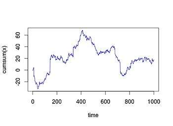
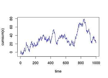
The importance of seven states of randomness classification for mathematical finance is that methods such as Markowitz mean variance portfolio and Black–Scholes model may be invalidated as the tails of the distribution of returns are fattened: the former relies on finite standard deviation (volatility) and stability of correlation, while the latter is constructed upon Brownian motion.
History
These seven states build on earlier work of Mandelbrot in 1963: "The variations of certain speculative prices"[2] and "New methods in statistical economics"[3] in which he argued that most statistical models approached only a first stage of dealing with indeterminism in science, and that they ignored many aspects of real world turbulence, in particular, most cases of financial modeling.[4][5] This was then presented by Mandelbrot in the International Congress for Logic (1964) in an address titled "The Epistemology of Chance in Certain Newer Sciences"[6]
Intuitively speaking, Mandelbrot argued[6] that the traditional normal distribution does not properly capture empirical and "real world" distributions and there are other forms of randomness that can be used to model extreme changes in risk and randomness. He observed that randomness can become quite "wild" if the requirements regarding finite mean and variance are abandoned. Wild randomness corresponds to situations in which a single observation, or a particular outcome can impact the total in a very disproportionate way.
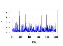
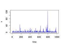
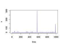
The classification was formally introduced in his 1997 book Fractals and Scaling in Finance,[1] as a way to bring insight into the three main states of randomness: mild, slow, and wild . Given N addends, portioning concerns the relative contribution of the addends to their sum. By even portioning, Mandelbrot meant that the addends were of same order of magnitude, otherwise he considered the portioning to be concentrated. Given the moment of order q of a random variable, Mandelbrot called the root of degree q of such moment the scale factor (of order q).
The seven states are:
- Proper mild randomness: short-run portioning is even for N = 2, e.g. the normal distribution
- Borderline mild randomness: short-run portioning is concentrated for N = 2, but eventually becomes even as N grows, e.g. the exponential distribution with rate λ = 1 (and so with expected value 1/λ = 1)
- Slow randomness with finite delocalized moments: scale factor increases faster than q but no faster than , w < 1
- Slow randomness with finite and localized moments: scale factor increases faster than any power of q, but remains finite, e.g. the lognormal distribution
- Pre-wild randomness: scale factor becomes infinite for q > 2, e.g. the Pareto distribution with α = 2.5
- Wild randomness: infinite second moment, but finite moment of some positive order, e.g. the Pareto distribution with
- Extreme randomness: all moments are infinite, e.g. the Log-Cauchy distribution
Wild randomness has applications outside financial markets, e.g. it has been used in the analysis of turbulent situations such as wild forest fires.[7]
Using elements of this distinction, in March 2006, a year before the Financial crisis of 2007–2010, and four years before the Flash crash of May 2010, during which the Dow Jones Industrial Average had a 1,000 point intraday swing within minutes,[8] Mandelbrot and Nassim Taleb published an article in the Financial Times arguing that the traditional "bell curves" that have been in use for over a century are inadequate for measuring risk in financial markets, given that such curves disregard the possibility of sharp jumps or discontinuities. Contrasting this approach with the traditional approaches based on random walks, they stated:[9]
We live in a world primarily driven by random jumps, and tools designed for random walks address the wrong problem.
Mandelbrot and Taleb pointed out that although one can assume that the odds of finding a person who is several miles tall are extremely low, similar excessive observations can not be excluded in other areas of application. They argued that while traditional bell curves may provide a satisfactory representation of height and weight in the population, they do not provide a suitable modeling mechanism for market risks or returns, where just ten trading days represent 63 per cent of the returns of the past 50 years.
Definitions
Doubling convolution
If the probability density of is denoted , then it can be obtained by the double convolution .
Short run portioning ratio
When u is known, the conditional probability density of u' is given by the portioning ratio:
Concentration in mode
In many important cases, the maximum of occurs near , or near and . Take the logarithm of and write:
- If is cap-convex, the portioning ratio is maximal for
- If is straight, the portioning ratio is constant
- If is cup-convex, the portioning ratio is minimal for
Concentration in probability
Splitting the doubling convolution in 3 parts gives:
p(u) is short-run concentrated in probability if it is possible to select so that the middle interval of () has the following two properties as u→∞:
- I0/p2(u) → 0
- does not → 0
Localized and delocalized moments
Consider the formula , if p(u) is the scaling distribution the integrand is maximum at 0 and ∞, on other cases the integrand may have a sharp global maximum for some value defined by the following equation:
One must also know in the neighborhood of . The function often admits a "Gaussian" approximation given by:
When is well-approximated by a Gaussian density, the bulk of originates in the "q-interval" defined as . The Gaussian q-intervals greatly overlap for all values of . The Gaussian moments are called delocalized. The lognormal's q-intervals are uniformly spaced and their width is independent of q; therefore if the log-normal is sufficiently skew, the q-interval and (q+1)-interval do not overlap. The lognormal moments are called uniformly localized. In other cases, neighboring q-intervals cease to overlap for sufficiently high q, such moments are called asymptotically localized.
The seven states of randomness
- Proper mild randomness: Short-run portioning is even for N=2.
- Borderline mild randomness: Short-run portioning is concentrated for N=2, but becomes even when N exceeds some finite threshold.
- Slow randomness with finite and delocalized moments: loosely characterized by either increasing faster than but no faster than , with w<1 or by increasing faster than q but no faster than a power of .
- Slow randomness with finite and localized moments: loosely characterized by either increasing faster than any power but less rapidly than any function of the form with γ<1, or by increasing faster than any power of q, but remaining finite.
- Pre-wild randomness: loosely characterized by increasing more rapidly than any functions of the form with γ<1 but less rapidly than or by being infinite when q≥α≥2.
- Wild randomness: characterized by , but for some q>0, however small.
- Extreme randomness: characterized by for all q>0.
See also
- History of randomness
- Random sequence
- Fat-tailed distribution
- Heavy-tailed distribution
- Daubechies wavelet for a system based on infinite moments (chaotic waves)
References
- Benoît Mandelbrot (1997) Fractals and scaling in finance ISBN 0-387-98363-5 pages 136–142 https://books.google.com/books/about/Fractals_and_Scaling_in_Finance.html?id=6KGSYANlwHAC&redir_esc=y
- B. Mandelbrot, The variation of certain Speculative Prices, The Journal of Business 1963
- B. Mandelbrot, New methods in statistical economics, The Journal of Political Economy 1963 https://www.jstor.org/stable/1829014
- Benoit Mandelbrot, F.J. Damerau, M. Frame, and K. McCamy (2001) Gaussian Self-Affinity and Fractals ISBN 0-387-98993-5 page 20
- Philip Mirowski (2004) The effortless economy of science? ISBN 0-8223-3322-8 page 255
- B. Mandelbrot, Toward a second stage of indeterminism in Science, Interdisciplinary Science Reviews 1987
- The Economics of Forest Disturbances: Wildfires, Storms and Invasive Species by Thomas P. Holmes, Jeffrey P. Prestemon, and Karen L. Abt. 2008. Springer: Dordrecht, The Netherlands. 422 p. ISBN 978-1-4020-4369-7
- Wall Street Journal May 11, 2010
- Benoît Mandelbrot and Nassim Taleb (23 March 2006), "A focus on the exceptions that prove the rule", Financial Times.