Regression-kriging
In applied statistics, regression-kriging (RK) is a spatial prediction technique that combines a regression of the dependent variable on auxiliary variables (such as parameters derived from digital elevation modelling, remote sensing/imagery, and thematic maps) with kriging of the regression residuals. It is mathematically equivalent to the interpolation method variously called universal kriging and kriging with external drift, where auxiliary predictors are used directly to solve the kriging weights.[1]
BLUP for spatial data

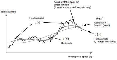
Regression-kriging is an implementation of the best linear unbiased predictor (BLUP) for spatial data, i.e. the best linear interpolator assuming the universal model of spatial variation. Matheron (1969) proposed that a value of a target variable at some location can be modeled as a sum of the deterministic and stochastic components:[2]
which he termed universal model of spatial variation. Both deterministic and stochastic components of spatial variation can be modeled separately. By combining the two approaches, we obtain:
where is the fitted deterministic part, is the interpolated residual, are estimated deterministic model coefficients ( is the estimated intercept), are kriging weights determined by the spatial dependence structure of the residual and where is the residual at location . The regression coefficients can be estimated from the sample by some fitting method, e.g. ordinary least squares (OLS) or, optimally, using generalized least squares (GLS):[3]
where is the vector of estimated regression coefficients, is the covariance matrix of the residuals, is a matrix of predictors at the sampling locations and is the vector of measured values of the target variable. The GLS estimation of regression coefficients is, in fact, a special case of the geographically weighted regression. In the case, the weights are determined objectively to account for the spatial auto-correlation between the residuals.
Once the deterministic part of variation has been estimated (regression-part), the residual can be interpolated with kriging and added to the estimated trend. The estimation of the residuals is an iterative process: first the deterministic part of variation is estimated using OLS, then the covariance function of the residuals is used to obtain the GLS coefficients. Next, these are used to re-compute the residuals, from which an updated covariance function is computed, and so on. Although this is by many geostatisticians recommended as the proper procedure, Kitanidis (1994) showed that use of the covariance function derived from the OLS residuals (i.e. a single iteration) is often satisfactory, because it is not different enough from the function derived after several iterations; i.e. it does not affect much the final predictions. Minasny and McBratney (2007) report similar results—it seems that using more higher quality data is more important than to use more sophisticated statistical methods.[4]
In matrix notation, regression-kriging is commonly written as:[5]
where is the predicted value at location , is the vector of predictors and is the vector of kriging weights used to interpolate the residuals. The RK model is considered to be the Best Linear Predictor of spatial data.[5][6] It has a prediction variance that reflects the position of new locations (extrapolation) in both geographical and feature space:
where is the sill variation and is the vector of covariances of residuals at the unvisited location.

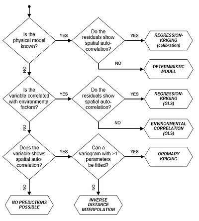
Many (geo)statisticians believe that there is only one Best Linear Unbiased Prediction model for spatial data (e.g. regression-kriging), all other techniques such as ordinary kriging, environmental correlation, averaging of values per polygons or inverse distance interpolation can be seen as its special cases. If the residuals show no spatial auto-correlation (pure nugget effect), the regression-kriging converges to pure multiple linear regression, because the covariance matrix () becomes an identity matrix. Likewise, if the target variable shows no correlation with the auxiliary predictors, the regression-kriging model reduces to ordinary kriging model because the deterministic part equals the (global) mean value. Hence, pure kriging and pure regression should be considered as only special cases of regression-kriging (see figure).
RK and UK/KED
The geostatistical literature uses many different terms for what are essentially the same or at least very similar techniques. This confuses the users and distracts them from using the right technique for their mapping projects. In fact, both universal kriging, kriging with external drift, and regression-kriging are basically the same technique.
Matheron (1969) originally termed the technique Le krigeage universel, however, the technique was intended as a generalized case of kriging where the trend is modelled as a function of coordinates. Thus, many authors reserve the term universal kriging (UK) for the case when only the coordinates are used as predictors. If the deterministic part of variation (drift) is defined externally as a linear function of some auxiliary variables, rather than the coordinates, the term kriging with external drift (KED) is preferred (according to Hengl 2007, "About regression-kriging: From equations to case studies"). In the case of UK or KED, the predictions are made as with kriging, with the difference that the covariance matrix of residuals is extended with the auxiliary predictors. However, the drift and residuals can also be estimated separately and then summed. This procedure was suggested by Ahmed et al. (1987) and Odeh et al. (1995) later named it regression-kriging, while Goovaerts (1997) uses the term kriging with a trend model to refer to a family of interpolators, and refers to RK as simple kriging with varying local means. Minasny and McBratney (2007) simply call this technique Empirical Best Linear Unbiased Predictor i.e. E-BLUP.[7][8][9][4]
In the case of KED, predictions at new locations are made by:
for
for or in matrix notation:
where is the target variable, 's are the predictor variables i.e. values at a new location , is the vector of KED weights (), is the number of predictors and is the vector of observations at primary locations. The KED weights are solved using the extended matrices:
where is the vector of solved weights, are the Lagrange multipliers, is the extended covariance matrix of residuals and is the extended vector of covariances at new location.
In the case of KED, the extended covariance matrix of residuals looks like this (Webster and Oliver, 2007; p. 183):[10]
and like this:
Hence, KED looks exactly as ordinary kriging, except the covariance matrix/vector are extended with values of auxiliary predictors.
Although the KED seems, at first glance, to be computationally more straightforward than RK, the parameters of the variogram for KED must also be estimated from regression residuals, thus requiring a separate regression modelling step. This regression should be GLS because of the likely spatial correlation between residuals. Note that many analyst use instead the OLS residuals, which may not be too different from the GLS residuals. However, they are not optimal if there is any spatial correlation, and indeed they may be quite different for clustered sample points or if the number of samples is relatively small ().
A limitation of KED is the instability of the extended matrix in the case that the covariate does not vary smoothly in space. RK has the advantage that it explicitly separates trend estimation from spatial prediction of residuals, allowing the use of arbitrarily-complex forms of regression, rather than the simple linear techniques that can be used with KED. In addition, it allows the separate interpretation of the two interpolated components. The emphasis on regression is important also because fitting of the deterministic part of variation (regression) is often more beneficial for the quality of final maps than fitting of the stochastic part (residuals).
Software to run regression-kriging

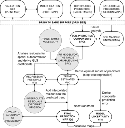
Regression-kriging can be automated e.g. in R statistical computing environment, by using gstat and/or geoR package. Typical inputs/outputs include:
INPUTS:
- Interpolation set (point map) — at primary locations;
- Minimum and maximum expected values and measurement precision ();
- Continuous predictors (raster map) — ; at new unvisited locations
- Discrete predictors (polygon map);
- Validation set (point map) — (optional);
- Lag spacing and limiting distance (required to fit the variogram);
OUTPUTS:
- Map of predictions and relative prediction error;
- Best subset of predictors and correlation significance (adjusted R-square);
- Variogram model parameters (e.g. , , )
- GLS drift model coefficients;
- Accuracy of prediction at validation points: mean prediction error (MPE) and root mean square prediction error (RMSPE);
Application of regression-kriging
Regression-kriging is used in various applied fields, from meteorology, climatology, soil mapping, geological mapping, species distribution modeling and similar. The only requirement for using regression-kriging versus e.g. ordinary kriging is that one or more covariate layers exist, and which are significantly correlated with the feature of interest. Some general applications of regression-kriging are:
- Geostatistical mapping: Regression-kriging allows for use of hybrid geostatistical techniques to model e.g. spatial distribution of soil properties.
- Downscaling of maps: Regression-kriging can be used a framework to downscale various existing gridded maps. In this case the covariate layers need to be available at better resolution (which corresponds to the sampling intensity) than the original point data.[11]
- Error propagation: Simulated maps generated by using a regression-kriging model can be used for scenario testing and for estimating propagated uncertainty.

Regression-kriging-based algorithms play more and more important role in geostatistics because the number of possible covariates is increasing every day.[1] For example, DEMs are now available from a number of sources. Detailed and accurate images of topography can now be ordered from remote sensing systems such as SPOT and ASTER; SPOT5 offers the High Resolution Stereoscopic (HRS) scanner, which can be used to produce DEMs at resolutions of up to 5 m.[12] Finer differences in elevation can also be obtained with airborne laser-scanners. The cost of data is either free or dropping in price as technology advances. NASA recorded most of the world's topography in the Shuttle Radar Topographic Mission in 2000.[13] From summer of 2004, these data has been available (e.g. via USGS ftp) for almost whole globe at resolution of about 90 m (for the North American continent at resolution of about 30 m). Likewise, MODIS multispectral images are freely available for download at resolutions of 250 m. A large free repository of Landsat images is also available for download via the Global Land Cover Facility (GLCF).
References
- Pebesma, Edzer J (1 July 2006). "The Role of External Variables and GIS Databases in Geostatistical Analysis" (PDF). Transactions in GIS. 10 (4): 615–632. doi:10.1111/j.1467-9671.2006.01015.x.
- Matheron, Georges (1969). "Part 1 of Cahiers du Centre de morphologie mathématique de Fontainebleau". Le krigeage universel. École nationale supérieure des mines de Paris.
- Cressie, Noel (2012). Statistics for spatio-temporal data. Hoboken, N.J.: Wiley. ISBN 9780471692744.
- Minasny, Budiman; McBratney, Alex B. (31 July 2007). "Spatial prediction of soil properties using EBLUP with the Matérn covariance function". Geoderma. 140 (4): 324–336. doi:10.1016/j.geoderma.2007.04.028.
- Christensen, Ronald (2001). Advanced linear modeling : multivariate, time series, and spatial data; nonparametric regression and response surface maximization (2. ed.). New York, NY [u.a.]: Springer. ISBN 9780387952963.
- Goldberger, A.S. (1962). "Best Linear Unbiased Prediction in the Generalized Linear Regression Model". Journal of the American Statistical Association. 57 (298): 369–375. doi:10.1080/01621459.1962.10480665. JSTOR 2281645.
- Ahmed, Shakeel; De Marsily, Ghislain (1 January 1987). "Comparison of geostatistical methods for estimating transmissivity using data on transmissivity and specific capacity". Water Resources Research. 23 (9): 1717. doi:10.1029/WR023i009p01717.
- Odeh, I.O.A.; McBratney, A.B.; Chittleborough, D.J. (31 July 1995). "Further results on prediction of soil properties from terrain attributes: heterotopic cokriging and regression-kriging". Geoderma. 67 (3–4): 215–226. doi:10.1016/0016-7061(95)00007-B.
- Hengl, Tomislav; Heuvelink, Gerard B.M.; Stein, Alfred (30 April 2004). "A generic framework for spatial prediction of soil variables based on regression-kriging" (PDF). Geoderma. 120 (1–2): 75–93. doi:10.1016/j.geoderma.2003.08.018.
- Webster, Richard; Oliver, Margaret A. (2007). Geostatistics for environmental scientists (2nd ed.). Chichester: Wiley. ISBN 9780470028582.
- Hengl, Tomislav; Bajat, Branislav; Blagojević, Dragan; Reuter, Hannes I. (1 December 2008). "Geostatistical modeling of topography using auxiliary maps" (PDF). Computers & Geosciences. 34 (12): 1886–1899. doi:10.1016/j.cageo.2008.01.005.
- Toutin, Thierry (30 April 2006). "Generation of DSMs from SPOT-5 in-track HRS and across-track HRG stereo data using spatiotriangulation and autocalibration". ISPRS Journal of Photogrammetry and Remote Sensing. 60 (3): 170–181. doi:10.1016/j.isprsjprs.2006.02.003.
- Rabus, Bernhard; Eineder, Michael; Roth, Achim; Bamler, Richard (31 January 2003). "The shuttle radar topography mission—a new class of digital elevation models acquired by spaceborne radar". ISPRS Journal of Photogrammetry and Remote Sensing. 57 (4): 241–262. doi:10.1016/S0924-2716(02)00124-7.
Further reading
- Chapter 2, Regression-kriging, in Tomislav Hengl (2009), A Practical Guide to Geostatistical Mapping, 291 p., ISBN 978-90-9024981-0.
- Hengl T., Heuvelink G. B. M., Rossiter D. G. (2007). "About regression-kriging: from equations to case studies". Computers & Geosciences. 33 (10): 1301–1315. doi:10.1016/j.cageo.2007.05.001.CS1 maint: uses authors parameter (link)