Radial basis function

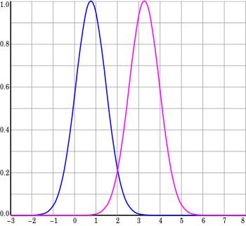
A radial basis function (RBF) is a real-valued function ${\textstyle \varphi }$ whose value depends only on the distance between the input and some fixed point, either the origin, so that ${\textstyle \varphi (\mathbf {x} )=\varphi (\left\|\mathbf {x} \right\|)}$, or some other fixed point ${\textstyle \mathbf {c} }$, called a center, so that ${\textstyle \varphi (\mathbf {x} )=\varphi (\left\|\mathbf {x} -\mathbf {c} \right\|)}$. Any function ${\textstyle \varphi }$ that satisfies the property ${\textstyle \varphi (\mathbf {x} )=\varphi (\left\|\mathbf {x} \right\|)}$ is a radial function. The distance is usually Euclidean distance, although other metrics are sometimes used. They are often used as a collection ${\displaystyle \{\varphi _{k}\}_{k}}$which forms a basis for some function space of interest, hence the name.

Sums of radial basis functions are typically used to approximate given functions. This approximation process can also be interpreted as a simple kind of neural network; this was the context in which they were originally applied to machine learning, in work by David Broomhead and David Lowe in 1988,[1][2] which stemmed from Michael J. D. Powell's seminal research from 1977.[3][4][5] RBFs are also used as a kernel in support vector classification.[6] The technique has proven effective and flexible enough that radial basis functions are now applied in a variety of engineering applications.[7][8]

Definition

A radial function is a function ${\textstyle \varphi$ :[0,\infty )\to \mathbb {R} } . When paired with a metric on a vector space ${\textstyle \|\cdot \|:V\to [0,\infty )}$ a function ${\textstyle \varphi _{\mathbf {c} }=\varphi (\|\mathbf {x} -\mathbf {c} \|)}$ is said to be a radial kernel centered at ${\textstyle \mathbf {c} }$. A Radial function and the associated radial kernels are said to be radial basis functions if, for any set of nodes ${\displaystyle \{\mathbf {x} _{k}\}_{k=1}^{n}}$

• The kernels ${\displaystyle \varphi _{\mathbf {x} _{1}},\varphi _{\mathbf {x} _{2}},\dots ,\varphi _{\mathbf {x} _{n}}}$ are linearly independent (for example ${\displaystyle \varphi (r)=r^{2}}$ in ${\displaystyle V=\mathbb {R} }$ is not a radial basis function)

• The kernels ${\displaystyle \varphi _{\mathbf {x} _{1}},\varphi _{\mathbf {x} _{2}},\dots ,\varphi _{\mathbf {x} _{n}}}$ form a basis for a Haar Space, meaning that the interpolation matrix

$${\displaystyle {\begin{bmatrix}\varphi (\|\mathbf {x} _{1}-\mathbf {x} _{1}\|)&\varphi (\|\mathbf {x} _{2}-\mathbf {x} _{1}\|)&\dots &\varphi (\|\mathbf {x} _{n}-\mathbf {x} _{1}\|)\\\varphi (\|\mathbf {x} _{1}-\mathbf {x} _{2}\|)&\varphi (\|\mathbf {x} _{2}-\mathbf {x} _{2}\|)&\dots &\varphi (\|\mathbf {x} _{n}-\mathbf {x} _{2}\|)\\\vdots &\vdots &\ddots &\vdots \\\varphi (\|\mathbf {x} _{1}-\mathbf {x} _{n}\|)&\varphi (\|\mathbf {x} _{2}-\mathbf {x} _{n}\|)&\dots &\varphi (\|\mathbf {x} _{n}-\mathbf {x} _{n}\|)\\\end{bmatrix}}}$$

is non-singular. [9] [10]

Examples

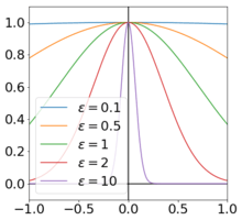
Commonly used types of radial basis functions include (writing ${\textstyle r=\left\|\mathbf {x} -\mathbf {x} _{i}\right\|}$ and using ${\textstyle \varepsilon }$ to indicate a shape parameter that can be used to scale the input of the radial kernel[11]):

• Infinitely Smooth RBFs

These radial basis functions are from ${\displaystyle C^{\infty }(\mathbb {R} )}$ and are strictly positive definite functions[12] that require tuning a shape parameter ${\displaystyle \varepsilon }$

• Gaussian:
  $${\displaystyle \varphi (r)=e^{-(\varepsilon r)^{2}}}$$

  

A Gaussian function for several choices of ${\displaystyle \varepsilon }$.

A plot of the scaled Bump function with several choices of ${\displaystyle \varepsilon }$.

• Multiquadric:
  $${\displaystyle \varphi (r)={\sqrt {1+(\varepsilon r)^{2}}}}$$

  

• Inverse quadratic:
  $${\displaystyle \varphi (r)={\dfrac {1}{1+(\varepsilon r)^{2}}}}$$

  

• Inverse multiquadric:
  $${\displaystyle \varphi (r)={\dfrac {1}{\sqrt {1+(\varepsilon r)^{2}}}}}$$

  

• Polyharmonic spline:
  $${\displaystyle {\begin{aligned}\varphi (r)&=r^{k},&k&=1,3,5,\dotsc \\\varphi (r)&=r^{k}\ln(r),&k&=2,4,6,\dotsc \end{aligned}}}$$

  
  *For even-degree polyharmonic splines ${\displaystyle (k=2,4,6,\dotsc )}$, to avoid numerical problems at ${\displaystyle r=0}$ where ${\displaystyle \ln(0)=-\infty }$, the computational implementation is often written as ${\displaystyle \varphi (r)=r^{k-1}\ln(r^{r})}$.

• Thin plate spline (a special polyharmonic spline):
  $${\displaystyle \varphi (r)=r^{2}\ln(r)}$$

  

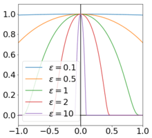
• Compactly Supported RBFs

These RBFs are compactly supported and thus are non-zero only within a radius of ${\displaystyle 1/\varepsilon }$, and thus have sparse differentiation matrices

• Bump function:

$${\displaystyle \varphi (r)={\begin{cases}\exp \left(-{\frac {1}{1-(\varepsilon r)^{2}}}\right)&{\mbox{ for }}r<{\frac {1}{\varepsilon }}\\0&{\mbox{ otherwise}}\end{cases}}}$$

Approximation

Main article: Radial basis function interpolation

Radial basis functions are typically used to build up function approximations of the form

$${\displaystyle y(\mathbf {x} )=\sum _{i=1}^{N}w_{i}\,\varphi (\left\|\mathbf {x} -\mathbf {x} _{i}\right\|),}$$

where the approximating function ${\textstyle y(\mathbf {x} )}$ is represented as a sum of ${\displaystyle N}$ radial basis functions, each associated with a different center ${\textstyle \mathbf {x} _{i}}$, and weighted by an appropriate coefficient ${\textstyle w_{i}.}$ The weights ${\textstyle w_{i}}$ can be estimated using the matrix methods of linear least squares, because the approximating function is linear in the weights ${\textstyle w_{i}}$.

Approximation schemes of this kind have been particularly used in time series prediction and control of nonlinear systems exhibiting sufficiently simple chaotic behaviour and 3D reconstruction in computer graphics (for example, hierarchical RBF and Pose Space Deformation).

RBF Network

Main article: radial basis function network

Two unnormalized Gaussian radial basis functions in one input dimension. The basis function centers are located at ${\textstyle x_{1}=0.75}$ and ${\textstyle x_{2}=3.25}$.

The sum

$${\displaystyle y(\mathbf {x} )=\sum _{i=1}^{N}w_{i}\,\varphi (\left\|\mathbf {x} -\mathbf {x} _{i}\right\|),}$$

can also be interpreted as a rather simple single-layer type of artificial neural network called a radial basis function network, with the radial basis functions taking on the role of the activation functions of the network. It can be shown that any continuous function on a compact interval can in principle be interpolated with arbitrary accuracy by a sum of this form, if a sufficiently large number ${\textstyle N}$ of radial basis functions is used.

The approximant ${\textstyle y(\mathbf {x} )}$ is differentiable with respect to the weights ${\textstyle w_{i}}$. The weights could thus be learned using any of the standard iterative methods for neural networks.

Using radial basis functions in this manner yields a reasonable interpolation approach provided that the fitting set has been chosen such that it covers the entire range systematically (equidistant data points are ideal). However, without a polynomial term that is orthogonal to the radial basis functions, estimates outside the fitting set tend to perform poorly.

See also

• Matérn covariance function
• Radial basis function interpolation

References

1. Radial Basis Function networks Archived 2014-04-23 at the Wayback Machine
2. Broomhead, David H.; Lowe, David (1988). "Multivariable Functional Interpolation and Adaptive Networks" (PDF). Complex Systems. 2: 321–355. Archived from the original (PDF) on 2014-07-14.
3. Michael J. D. Powell (1977). "Restart procedures for the conjugate gradient method". Mathematical Programming. 12 (1): 241–254. doi:10.1007/bf01593790.
4. Sahin, Ferat (1997). A Radial Basis Function Approach to a Color Image Classification Problem in a Real Time Industrial Application (PDF) (M.Sc.). Virginia Tech. p. 26. Radial basis functions were first introduced by Powell to solve the real multivariate interpolation problem.
5. Broomhead & Lowe 1988, p. 347: "We would like to thank Professor M.J.D. Powell at the Department of Applied Mathematics and Theoretical Physics at Cambridge University for providing the initial stimulus for this work."
6. VanderPlas, Jake (6 May 2015). "Introduction to Support Vector Machines". [O'Reilly]. Retrieved 14 May 2015.
7. Buhmann, Martin Dietrich (2003). Radial basis functions : theory and implementations. Cambridge University Press. ISBN 978-0511040207. OCLC 56352083.
8. Biancolini, Marco Evangelos (2018). Fast radial basis functions for engineering applications. Springer International Publishing. ISBN 9783319750118. OCLC 1030746230.
9. Fasshauer, Gregory E. (2007). Meshfree Approximation Methods with MATLAB. Singapore: World Scientific Publishing Co. Pte. Ltd. pp. 17–25. ISBN 9789812706331.
10. Wendland, Holger (2005). Scattered Data Approximation. Cambridge: Cambridge University Press. pp. 11, 18–23, 64–66. ISBN 0521843359.
11. Fasshauer, Gregory E. (2007). Meshfree Approximation Methods with MATLAB. Singapore: World Scientific Publishing Co. Pte. Ltd. p. 37. ISBN 9789812706331.
12. Fasshauer, Gregory E. (2007). Meshfree Approximation Methods with MATLAB. Singapore: World Scientific Publishing Co. Pte. Ltd. pp. 37–45. ISBN 9789812706331.

Further reading

• Hardy, R.L. (1971). "Multiquadric equations of topography and other irregular surfaces". Journal of Geophysical Research. 76 (8): 1905–1915. Bibcode:1971JGR....76.1905H. doi:10.1029/jb076i008p01905.
• Hardy, R.L. (1990). "Theory and applications of the multiquadric-biharmonic method, 20 years of Discovery, 1968 1988". Comp. Math Applic. 19 (8/9): 163–208. doi:10.1016/0898-1221(90)90272-l.
• Press, WH; Teukolsky, SA; Vetterling, WT; Flannery, BP (2007), "Section 3.7.1. Radial Basis Function Interpolation", Numerical Recipes: The Art of Scientific Computing (3rd ed.), New York: Cambridge University Press, ISBN 978-0-521-88068-8
• Sirayanone, S., 1988, Comparative studies of kriging, multiquadric-biharmonic, and other methods for solving mineral resource problems, PhD. Dissertation, Dept. of Earth Sciences, Iowa State University, Ames, Iowa.
• Sirayanone, S.; Hardy, R.L. (1995). "The Multiquadric-biharmonic Method as Used for Mineral Resources, Meteorological, and Other Applications". Journal of Applied Sciences and Computations. 1: 437–475.