Parallel all-pairs shortest path algorithm

A central problem in algorithmic graph theory is the shortest path problem. Hereby, the problem of finding the shortest path between every pair of nodes is known as all-pair-shortest-paths (APSP) problem. As sequential algorithms for this problem often yield long runtimes, parallelization has shown to be beneficial in this field. In this article two efficient algorithms solving this problem are introduced.

Another variation of the problem is the single-source-shortest-paths (SSSP) problem, which also has parallel approaches: Parallel single-source shortest path algorithm.

Problem definition

Let ${\displaystyle G=(V,E,w)}$ be a directed Graph with the set of nodes ${\displaystyle V}$ and the set of edges ${\displaystyle E\subseteq V\times V}$. Each edge ${\displaystyle e\in E}$ has a weight ${\displaystyle w(e)}$ assigned. The goal of the all-pair-shortest-paths problem is to find the shortest path between all pairs of nodes of the graph. For this path to be unique it is required that the graph does not contain cycles with a negative weight.

In the remainder of the article it is assumed that the graph is represented using an adjacency matrix. We expect the output of the algorithm to be a distancematrix ${\displaystyle D}$. In ${\displaystyle D}$, every entry ${\displaystyle d-{i,j}}$ is the weight of the shortest path in ${\displaystyle G}$ from node ${\displaystyle i}$ to node ${\displaystyle j}$.

The Floyd algorithm presented later can handle negative edge weights, whereas the Dijkstra algorithm requires all edges to have a positive weight.

Dijkstra algorithm

The Dijkstra algorithm originally was proposed as a solver for the single-source-shortest-paths problem. However, the algorithm can easily be used for solving the All-Pair-Shortest-Paths problem by executing the Single-Source variant with each node in the role of the root node.

In pseudocode such an implementation could look as follows:

 1    func DijkstraSSSP(G,v) {
 2        ... //standard SSSP-implementation here
 3        return dv;
 4    }
 5    
 6    func DijkstraAPSP(G) {
 7        D := |V|x|V|-Matrix
 8        for i from 1 to |V| {
 9           //D[v] denotes the v-th row of D
 10          D[v] := DijkstraSSP(G,i)
 11       }
 12   }

In this example we assume that DisjktraSSSP takes the graph ${\displaystyle G}$ and the root node ${\displaystyle v}$ as input. The result of the execution in turn is the distancelist ${\displaystyle d_{v}}$. In ${\displaystyle d_{v}}$, the ${\displaystyle i}$-th element stores the distance from the root node ${\displaystyle v}$ to the node ${\displaystyle i}$. Therefore the list ${\displaystyle d_{v}}$ corresponds exactly to the ${\displaystyle v}$-th row of the APSP distancematrix ${\displaystyle D}$. For this reason, DijkstraAPSP iterates over all nodes of the graph ${\displaystyle G}$ and executes DisjktraSSSP with each as root node while storing the results in ${\displaystyle D}$.

The runtime of DijkstraSSSP is ${\displaystyle O(|V|^{2})}$ as we expect the graph to be represented using an adjacency matrix. Therefore DijkstraAPSP has a total sequential runtime of ${\displaystyle O(|V|^{3})}$.

Parallelization for up to |V| processors

A trivial parallelization can be obtained by parallelizing the loop of DijkstraAPSP in line8. However, when using the sequential DijkstraSSSP this limits the number of processors to be used by the number of iterations executed in the loop. Therefore, for this trivial parallelization ${\displaystyle |V|}$ is an upper bound for the number of processors.

For example, let the number of processors ${\displaystyle p}$ be equal to the number of nodes ${\displaystyle |V|}$. This results in each processor executing DijkstraSSSP exactly once in parallel. However, when there are only for example ${\displaystyle p={\frac {|V|}{2}}}$ processors available, each processor has to execute DijkstraSSSP twice.

In total this yields a runtime of ${\displaystyle O(|V|^{2}\cdot {\frac {|V|}{p}})}$, when ${\displaystyle |V|}$ is a multiple of ${\displaystyle p}$. Consequently, the efficiency of this parallelization is perfect: Employing ${\displaystyle p}$ processors reduces the runtime by the factor ${\displaystyle p}$.

Another benefit of this parallelization is that no communication between the processors is required. However, it is required that every processor has enough local memory to store the entire adjacency matrix of the graph.

Parallelization for more than |V| processors

If more than ${\displaystyle |V|}$ processors shall be used for the parallelization, it is required that multiple processors take part of the DijkstraSSSP computation. For this reason, the parallelization is split across into two levels.

For the first level the processors are split into ${\displaystyle |V|}$ partitions. Each partition is responsible for the computation of a single row of the distancematrix ${\displaystyle D}$. This means each partition has to evaluate one DijkstraSSSP execution with a fixed root node. With this definition each partition has a size of ${\displaystyle k={\frac {p}{|V|}}}$ processors. The partitions can perform their computations in parallel as the results of each are independent of each other. Therefore, the parallelization presented in the previous section corresponds to a partition size of 1 with ${\displaystyle p=|V|}$ processors.

The main difficulty is the parallelization of multiple processors executing DijkstraSSSP for a single root node. The idea for this parallelization is to distribute the management of the distancelist ${\displaystyle d_{v}}$ in DijkstraSSSP within the partition. Each processor in the partition therefore is exclusively responsible for ${\displaystyle {\frac {|V|}{k}}}$ elements of ${\displaystyle d_{v}}$. For example, consider ${\displaystyle |V|=4}$ and ${\displaystyle p=8}$: this yields a partition size of ${\displaystyle k=2}$. In this case, the first processor of each partition is responsible for ${\displaystyle d_{v,1}}$, ${\displaystyle d_{v,2}}$ and the second processor is responsible for ${\displaystyle d_{v,3}}$ and ${\displaystyle d_{v,4}}$. Hereby, the total distance lists is ${\displaystyle d_{v}=[d_{v,1},d_{v,2},d_{v,3},d_{v,4}]}$.

The DijkstraSSSP algorithm mainly consists of the repetition of two steps: First, the nearest node ${\displaystyle x}$ in the distancelist ${\displaystyle d_{v}}$ has to be found. For this node the shortest path already has been found. Afterwards the distance of all neighbors of ${\displaystyle x}$ has to be adjusted in ${\displaystyle d_{v}}$.

These steps have to be altered as follows because for the parallelization ${\displaystyle d_{v}}$ has been distributed across the partition:

1. Find the node ${\displaystyle x}$ with the shortest distance in ${\displaystyle d_{v}}$.
   • Each processor owns a part of ${\displaystyle d_{v}}$: Each processor scans for the local minimum ${\displaystyle {\tilde {x}}}$ in his part, for example using linear search.
   • Compute the global minimum ${\displaystyle x}$ in ${\displaystyle d_{v}}$ by performing a reduce-operation across all ${\displaystyle {\tilde {x}}}$.
   • Broadcast the global minimum ${\displaystyle x}$ to all nodes in the partition.
2. Adjust the distance of all neighbors of ${\displaystyle x}$ in ${\displaystyle d_{v}}$
   • Every processors now knows the global nearest node ${\displaystyle x}$ and its distance. Based on this information, adjust the neighbors of ${\displaystyle x}$ in ${\displaystyle d_{v}}$ which are managed by the corresponding processor.

The total runtime of such an iteration of DijkstraSSSP performed by a partition of size ${\displaystyle k}$ can be derived based on the performed subtasks:

• The linear search for ${\displaystyle {\tilde {x}}}$: ${\displaystyle O({\frac {|V|}{k}})}$
• Broadcast- and Reduce-operations: These can be implemented efficiently for example using binonmialtrees. This yields a communication overhead of ${\displaystyle O(\log k)}$.

For ${\displaystyle |V|}$-iterations this results in a total runtime of ${\displaystyle O(|V|({\frac {|V|}{k}}+\log k))}$. After substituting the definition of ${\displaystyle k}$ this yields the total runtime for DijkstraAPSP: ${\displaystyle O({\frac {|V|^{3}}{p}}+\log p)}$.

The main benefit of this parallelization is that it is not required anymore that every processor stores the entire adjacency matrix. Instead, it is sufficient when each processor within a partition only stores the columns of the adjacency matrix of the nodes for which he is responsible. Given a partition size of ${\displaystyle k}$, each processor only has to store ${\displaystyle {\frac {|V|}{k}}}$ columns of the adjacency matrix. A downside, however, is that this parallelization comes with a communication overhead due to the reduce- and broadcast-operations.

Example

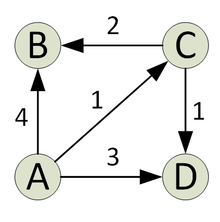
The graph used in this example is the one presented in the image with four nodes.

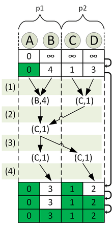
The goal is to compute the distancematrix with ${\displaystyle p=8}$ processors. For this reason, the processors are divided into four partitions with two processors each. For the illustration we focus on the partition which is responsible for the computation of the shortest paths from node A to all other nodes. Let the processors of this partition be named p1 and p2.

The computation of the distancelist across the different iterations is visualized in the second image.

The top row in the image corresponds to ${\displaystyle d_{A}}$ after the initialization, the bottom one to ${\displaystyle d_{A}}$ after the termination of the algorithm. The nodes are distributed in a way that p1 is responsible for the nodes A and B, while p2 is responsible for C and D. The distancelist ${\displaystyle d_{A}}$ is distributed according to this. For the second iteration the subtasks executed are shown explicitly in the image:

1. Computation of the local minimum node in ${\displaystyle d_{A}}$
2. Computation of the globalminimum node in ${\displaystyle d_{A}}$ through a reduce operation
3. Broadcast of the global minimum node in ${\displaystyle d_{A}}$
4. Marking of the global nearest node as "finished" and adjusting the distance of its neighbors

Floyd algorithm

The Floyd algorithm solves the All-Pair-Shortest-Paths problem for directed graphs. With the adjacency matrix of a graph as input, it calculates shorter paths iterative. After |V| iterations the distance-matrix contains all the shortest paths. The following describes a sequential version of the algorithm in pseudo code:

 1    func Floyd_All_Pairs_SP(A) {
 2        ${\displaystyle D^{(0)}}$ = A;
 3        for k := 1 to n do
 4            for i := 1 to n do
 5                for j := 1 to n do
 6                    ${\displaystyle d_{i,j}^{(k)}:=\min(d_{i,j}^{(k-1)},d_{i,k}^{(k-1)}+d_{k,j}^{(k-1)})}$
 7     }

partition of a matrix with 2-D block mapping

Where A is the adjacency matrix, n = |V| the number of nodes and D the distance matrix. For a more detailed description of the sequential algorithm look up Floyd–Warshall algorithm.

Parallelization

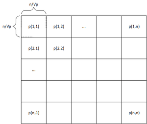
The basic idea to parallelize the algorithm is to partition the matrix and split the computation between the processes. Each process is assigned to a specific part of the matrix. A common way to achieve this is 2-D Block Mapping. Here the matrix is partitioned into squares of the same size and each square gets assigned to a process. For an ${\displaystyle n\times n}$-matrix and p processes each process calculates a ${\displaystyle n/{\sqrt {p}}\times n/{\sqrt {p}}}$ sized part of the distance matrix. For ${\displaystyle p=n^{2}}$ processes each would get assigned to exactly one element of the matrix. Because of that the parallelization only scales to a maximum of ${\displaystyle n^{2}}$ processes. In the following we refer with ${\displaystyle p_{i,j}}$ to the process that is assigned to the square in the i-th row and the j-th column.

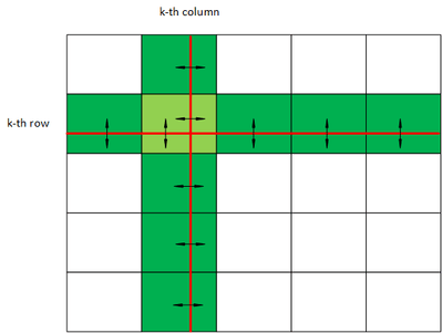
As the calculation of the parts of the distance matrix is dependent on results from other parts the processes have to communicate between each other and exchange data. In the following we refer with ${\displaystyle d_{i,j}^{(k)}}$ to the element of the i-th row and j-th column of the distance matrix after the k-th iteration. To calculate ${\displaystyle d_{i,j}^{(k)}}$ we need the elements ${\displaystyle d_{i,j}^{(k-1)}}$, ${\displaystyle d_{i,k}^{(k-1)}}$ and ${\displaystyle d_{k,j}^{(k-1)}}$ as specified in line 6 of the algorithm. ${\displaystyle d_{i,j}^{(k-1)}}$ is available to each process as it was calculated by itself in the previous iteration.

Additionally each process needs a part of the k-th row and the k-th column of the ${\displaystyle D^{k-1}}$ matrix. The ${\displaystyle d_{i,k}^{(k-1)}}$ element holds a process in the same row and the ${\displaystyle d_{k,j}^{(k-1)}}$ element holds a process in the same column as the process that wants to compute ${\displaystyle d_{i,j}^{(k)}}$. Each process that calculated a part of the k-th row in the ${\displaystyle D^{k-1}}$ matrix has to send this part to all processes in its column. Each process that calculated a part of the k-th column in the ${\displaystyle D^{k-1}}$ matrix has to send this part to all processes in its row. All this processes have to do a one-to-all-broadcast operation along the row or the column. The data dependencies are illustrated in the image below.

For the 2-D block mapping we have to modify the algorithm as follows:

 1    func Floyd_All_Pairs_Parallel(${\displaystyle D^{(0)}}$) {
 2      for k := 1 to n do{
 3          Each process ${\displaystyle p_{i,j}}$ that has a segment of the k-th row of ${\displaystyle D^{(k-1)}}$,
            broadcasts it to the ${\displaystyle p_{*,j}}$ processes;
 4          Each process ${\displaystyle p_{i,j}}$ that has a segment of the k-th column of ${\displaystyle D^{(k-1)}}$,
            broadcasts it to the ${\displaystyle p_{i,*}}$ processes;
 5          Each process waits to receive the needed segments;
 6          Each process computes its part of the ${\displaystyle D^{(k)}}$ matrix;
 7          }
 8     }

data dependencies in Floyd algorithm

In line 5 of the algorithm we have a synchronisation step to ensure that all processes have the data necessary to compute the next iteration. To improve the runtime of the algorithm we can remove the synchronisation step without affecting the correctness of the algorithm. To achieve that each process starts the computation as soon as it has the data necessary to compute its part of the matrix. This version of the algorithm is called pipelined 2-D block mapping.

Runtime

The runtime of the sequential algorithm is determined by the triple nested for loop. The computation in line 6 can be done in constant time (${\displaystyle O(1)}$). Therefore, the runtime of the sequential algorithm is ${\displaystyle O(n^{3})}$.

2-D block mapping

The runtime of the parallelized algorithm consists of two parts. The time for the computation and the part for communication and data transfer between the processes.

As there is no additional computation in the algorithm and the computation is split equally among the p processes, we have a runtime of ${\displaystyle O(n^{3}/p)}$ for the computational part.

In each iteration of the algorithm there is a one-to-all broadcast operation performed along the row and column of the processes. There are ${\displaystyle n/{\sqrt {p}}}$ elements broadcast. Afterwards there is a synchronisation step performed. How much time these operations take is highly dependent on the architecture of the parallel system used. Therefore, the time needed for communication and data transfer in the algorithm is ${\displaystyle T_{\text{comm}}=n(T_{\text{synch}}+T_{\text{broadcast}})}$.

For the whole algorithm we have the following runtime:

${\displaystyle T=O\left({\frac {n^{3}}{p}}\right)+n(T_{\text{synch}}+T_{\text{broadcast}})}$

Pipelined 2-D block mapping

For the runtime of the data transfer between the processes in the pipelined version of the algorithm we assume that a process can transfer k elements to a neighbouring process in ${\displaystyle O(k)}$ time. In every step there are ${\displaystyle n/{\sqrt {p}}}$ elements of a row or a column send to a neighbouring process. Such a step takes ${\displaystyle O(n/{\sqrt {p}})}$ time. After ${\displaystyle {\sqrt {p}}}$ steps the relevant data of the first row and column arrive at process ${\displaystyle p_{{\sqrt {p}},{\sqrt {p}}}}$ (in ${\displaystyle O(n)}$ time).

The values of successive rows and columns follow after time ${\displaystyle O(n^{2}/p)}$ in a pipelined mode. Process ${\displaystyle p_{{\sqrt {p}},{\sqrt {p}}}}$ finishes its last computation after O(${\displaystyle n^{3}/p}$) + O(${\displaystyle n}$) time. Therefore, the additional time needed for communication in the pipelined version is ${\displaystyle O(n)}$.

The overall runtime for the pipelined version of the algorithm is:

${\displaystyle T=O\left({\frac {n^{3}}{p}}\right)+O(n)}$

References

Bibliography

• Grama, A.: Introduction to parallel computing. Pearson Education, 2003.
• Kumar, V.: Scalability of Parallel Algorithms for the All-Pairs Shortest-Path Problem. Journal of Parallel and Distributed Programming 13, 1991.
• Foster, I.: Designing and Building Parallel Programs (Online).
• Bindell, Fall: Parallel All-Pairs Shortest Paths Applications of Parallel Computers, 2011.