Nagel–Schreckenberg model
The Nagel–Schreckenberg model is a theoretical model for the simulation of freeway traffic. The model was developed in the early 1990s by the German physicists Kai Nagel and Michael Schreckenberg.[1] It is essentially a simple cellular automaton model for road traffic flow that can reproduce traffic jams, i.e., show a slow down in average car speed when the road is crowded (high density of cars). The model shows how traffic jams can be thought of as an emergent or collective phenomenon due to interactions between cars on the road, when the density of cars is high and so cars are close to each other on average.
Outline of the model
In the Nagel–Schreckenberg model, a road is divided into cells. In the original model, these cells are aligned in a single row whose ends are connected so that all cells make up a circle (this is an example of what are called periodic boundary conditions). Each cell is either empty road or contains a single car; i.e., no more than one car can occupy a cell at any time. Each car is assigned a velocity which is an integer between 0 and a maximum velocity (= 5 in Nagel and Schreckenberg's original work).

Time is discretized into time steps. This discretization in both space and time results in a cellular automaton. One can think of a cell as being a few car lengths long and the maximum velocity as being the speed limit on the road. The time step is then the time taken for a car at the speed limit to travel around 10 car lengths. However, the model can also be thought as just a way to understand or to model features of traffic jams by showing how interactions between nearby cars cause the cars to slow down. In each time step, the procedure is as follows.[1]
In each step, the following four actions are conducted in order from first to last, and all are applied to all cars. In each action the updates are applied to all cars in parallel.
- Acceleration: All cars not at the maximum velocity have their velocity increased by one unit. For example, if the velocity is 4 it is increased to 5.
- Slowing down: All cars are checked to see if the distance between it and the car in front (in units of cells) is smaller than its current velocity (which has units of cells per time step). If the distance is smaller than the velocity, the velocity is reduced to the number of empty cells in front of the car – to avoid a collision. For example, if the velocity of a car is now 5, but there are only 3 free cells in front of it, with the fourth cell occupied by another car, the car velocity is reduced to 3.
- Randomization: The speed of all cars that have a velocity of at least 1, is now reduced by one unit with a probability of p. For example, if p = 0.5, then if the velocity is 4, it is reduced to 3 50% of the time.
- Car motion: Finally, all cars are moved forward the number of cells equal to their velocity. For example, if the velocity is 3, the car is moved forward 3 cells.
These four actions are repeated many times, as long as is required to study any traffic jams that may form. The model is an example of a cellular automaton. The model is for a single lane where cars cannot pass each other; there is no overtaking.
Example simulation in the state with traffic jams
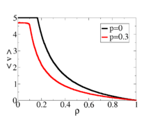
Above and to the right is a plot of the average velocity as a function of the density of cars, obtained from a simulation of the original Nagel–Schreckenberg model.[1] In the deterministic limit, p = 0, the velocity is constant at the maximum velocity (here 5) up to a density ρ = 1/(maximum velocity + 1) = 1 / 6 = 0.167, at which point there is a discontinuity in the slope due to the sudden appearance of traffic jams. Then as the density increases further, the average velocity decreases until it reaches zero when the road is 100% occupied. When p = 0.3, and so there are random decreases in velocity, then at low densities the average velocity is of course slower. However, note p > 0 also shifts the density at which jams appear to lower densities – traffic jams appear at the knee in the curve which for p = 0.3 is close to 0.15, and the random decelerations round off the discontinuity in the slope found for p = 0 at the onset of traffic jams.[2]

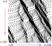
To the right is the result of an example simulation run of the Nagel–Schreckenberg model, with maximum velocity 5, density of cars 0.35 and probability of deceleration p = 0.3. It is a road of 100 cells. Cars are shown as black dots, and so, for example, if the road had a single car on it the plot would be white except for a single black line of slope −1/5 (maximum velocity = 5). The lines have slopes that are steeper, indicating that jamming is slowing the cars down. Small traffic jams show up as dark bands, i.e., groups of cars that are nose-to-tail and moving slowly to the right. The rippling of the bands is due to the randomization step.
So, the Nagel–Schreckenberg model includes the effect of cars getting in each other's way and so slowing each other down. The average velocity at this density is a little over 1, while at low density it is a little less than the maximum velocity of 5. It also shows that this is a collective phenomenon in which cars bunch up into traffic jams. When jamming occurs the distribution of cars along the road becomes highly non-uniform.
Role of randomization
Without the randomization step (third action), the model is a deterministic algorithm, i.e., the cars always move in a set pattern once the original state of the road is set. With randomization this is not the case, as it is on a real road with human drivers. Randomization has the effect of rounding off an otherwise sharp transition.[2] Just below this transition, one car braking due to a random slow can slow down the cars behind, spontaneously creating a jam. This feature of one car braking at random and causing a jam is absent in a deterministic model.
Model properties
- The model explains how traffic congestions can emerge without external influences, just because of crowding on a road.
- It was shown that variants of the Nagel–Schreckenberg model deliver (with a tolerance in the range of jam spacing) precisely the same results for vehicle trajectories as kinematic wave models and linear vehicle-following models.[3]
- For a maximum speed of one (instead of five) and no probability of slowing down, the model equals cellular automaton 184 by Stephen Wolfram.
- The model is minimalist, i.e. that the exclusion of any element of the model’s definition will immediately cause loss of crucial properties of traffic.
Application
- The Nagel–Schreckenberg model was further developed during Nagel's research stay at the Los Alamos National Laboratory for parallel computing. The transportation forecasting model Transims is based on this work.
- In the German state (bundesland) of North Rhine-Westphalia the Nagel–Schreckenberg model has been used as the foundation for a comprehensive traffic forecasting system which is accessibile online.
References
- Nagel, K.; Schreckenberg, M. (1992). "A cellular automaton model for freeway traffic" (PDF). Journal de Physique I. 2 (12): 2221. Bibcode:1992JPhy1...2.2221N. doi:10.1051/jp1:1992277. Archived from the original (PDF) on 2014-03-11.
- Eisenblätter, B.; Santen, L.; Schadschneider, A.; Schreckenberg, M. (1998). "Jamming transition in a cellular automaton model for traffic flow". Physical Review E. 57 (2): 1309. arXiv:cond-mat/9706041. Bibcode:1998PhRvE..57.1309E. doi:10.1103/PhysRevE.57.1309.
- Daganzo, C. F. (2006). "In traffic flow, cellular automata = kinematic waves" (PDF). Transportation Research Part B: Methodological. 40 (5): 396–403. doi:10.1016/j.trb.2005.05.004.