Monte Carlo integration

In mathematics, Monte Carlo integration is a technique for numerical integration using random numbers. It is a particular Monte Carlo method that numerically computes a definite integral. While other algorithms usually evaluate the integrand at a regular grid,[1] Monte Carlo randomly chooses points at which the integrand is evaluated.[2] This method is particularly useful for higher-dimensional integrals.[3]

An illustration of Monte Carlo integration. In this example, the domain D is the inner circle and the domain E is the square. Because the square's area (4) can be easily calculated, the area of the circle (π*1.0²) can be estimated by the ratio (0.8) of the points inside the circle (40) to the total number of points (50), yielding an approximation for the circle's area of 4*0.8 = 3.2 ≈ π.

There are different methods to perform a Monte Carlo integration, such as uniform sampling, stratified sampling, importance sampling, sequential Monte Carlo (also known as a particle filter), and mean field particle methods.

Overview

In numerical integration, methods such as the trapezoidal rule use a deterministic approach. Monte Carlo integration, on the other hand, employs a non-deterministic approach: each realization provides a different outcome. In Monte Carlo, the final outcome is an approximation of the correct value with respective error bars, and the correct value is likely to be within those error bars.

The problem Monte Carlo integration addresses the computation of a multidimensional definite integral

${\displaystyle I=\int _{\Omega }f({\overline {\mathbf {x} }})\,d{\overline {\mathbf {x} }}}$

where Ω, a subset of R^m, has volume

${\displaystyle V=\int _{\Omega }d{\overline {\mathbf {x} }}}$

The naive Monte Carlo approach is to sample points uniformly on Ω:[4] given N uniform samples,

${\displaystyle {\overline {\mathbf {x} }}_{1},\cdots ,{\overline {\mathbf {x} }}_{N}\in \Omega ,}$

I can be approximated by

${\displaystyle I\approx Q_{N}\equiv V{\frac {1}{N}}\sum _{i=1}^{N}f({\overline {\mathbf {x} }}_{i})=V\langle f\rangle }$.

This is because the law of large numbers ensures that

${\displaystyle \lim _{N\to \infty }Q_{N}=I}$.

Given the estimation of I from Q_N, the error bars of Q_N can be estimated by the sample variance using the unbiased estimate of the variance.

${\displaystyle \mathrm {Var} (f)\equiv \sigma _{N}^{2}={\frac {1}{N-1}}\sum _{i=1}^{N}\left(f({\overline {\mathbf {x} }}_{i})-\langle f\rangle \right)^{2}.}$

which leads to

${\displaystyle \mathrm {Var} (Q_{N})={\frac {V^{2}}{N^{2}}}\sum _{i=1}^{N}\mathrm {Var} (f)=V^{2}{\frac {\mathrm {Var} (f)}{N}}=V^{2}{\frac {\sigma _{N}^{2}}{N}}}$.

As long as the sequence

${\displaystyle \left\{\sigma _{1}^{2},\sigma _{2}^{2},\sigma _{3}^{2},\ldots \right\}}$

is bounded, this variance decreases asymptotically to zero as 1/N. The estimation of the error of Q_N is thus

${\displaystyle \delta Q_{N}\approx {\sqrt {\mathrm {Var} (Q_{N})}}=V{\frac {\sigma _{N}}{\sqrt {N}}},}$

which decreases as ${\displaystyle {\tfrac {1}{\sqrt {N}}}}$. This is standard error of the mean multiplied with ${\displaystyle V}$. This result does not depend on the number of dimensions of the integral, which is the promised advantage of Monte Carlo integration against most deterministic methods that depend exponentially on the dimension.[5] It is important to notice that, unlike in deterministic methods, the estimate of the error is not a strict error bound; random sampling may not uncover all the important features of the integrand that can result in an underestimate of the error.

While the naive Monte Carlo works for simple examples, an improvement over deterministic algorithms only can be accomplished with algorithms that use problem specific sampling distributions. With an appropriate sample distribution it is possible to exploit the fact that almost all higher-dimensional integrands are very localized and only small subspace notably contributes to the integral[6]. A large part of the Monte Carlo literature is dedicated in developing strategies to improve the error estimates. In particular, stratified sampling—dividing the region in sub-domains—, and importance sampling—sampling from non-uniform distributions—are two of such techniques.

Example

Relative error as a function of the number of samples, showing the scaling ${\displaystyle {\tfrac {1}{\sqrt {N}}}}$

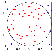
A paradigmatic example of a Monte Carlo integration is the estimation of π. Consider the function

${\displaystyle H\left(x,y\right)={\begin{cases}1&{\text{if }}x^{2}+y^{2}\leq 1\\0&{\text{else}}\end{cases}}}$

and the set Ω = [−1,1] × [−1,1] with V = 4. Notice that

${\displaystyle I_{\pi }=\int _{\Omega }H(x,y)dxdy=\pi .}$

Thus, a crude way of calculating the value of π with Monte Carlo integration is to pick N random numbers on Ω and compute

${\displaystyle Q_{N}=4{\frac {1}{N}}\sum _{i=1}^{N}H(x_{i},y_{i})}$

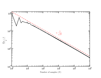
In the figure on the right, the relative error ${\displaystyle {\tfrac {Q_{N}-\pi }{\pi }}}$ is measured as a function of N, confirming the ${\displaystyle {\tfrac {1}{\sqrt {N}}}}$.

C example

Keep in mind that a true random number generator should be used.

int i, throws = 99999, insideCircle = 0;
double randX, randY, pi;

srand(time(NULL));

for (i = 0; i < throws; ++i) {
  randX = rand() / (double) RAND_MAX;
  randY = rand() / (double) RAND_MAX;
  if (randX * randX + randY * randY < 1) ++insideCircle;
}

pi = 4.0 * insideCircle / throws;

Wolfram Mathematica example

The code below describes a process of integrating the function

${\displaystyle f(x)={\frac {1}{1+\sinh(2x)\log(x)^{2}}}}$

from ${\displaystyle 0.8<x<3}$ using the Monte-Carlo method in Mathematica:

func[x_] := 1/(1 + Sinh[2*x]*(Log[x])^2);

(*Sample from truncated normal distribution to speed up convergence*)
Distrib[x_, average_, var_] :=   PDF[NormalDistribution[average, var], 1.1*x - 0.1];
n = 10;
RV = RandomVariate[TruncatedDistribution[{0.8, 3}, NormalDistribution[1, 0.399]], n];
Int = 1/n Total[func[RV]/Distrib[RV, 1, 0.399]]*Integrate[Distrib[x, 1, 0.399], {x, 0.8, 3}]

NIntegrate[func[x], {x, 0.8, 3}] (*Compare with real answer*)

Recursive stratified sampling

See also: Stratified sampling

An illustration of Recursive Stratified Sampling. In this example, the function: ${\displaystyle f(x,y)={\begin{cases}1&x^{2}+y^{2}<1\\0&x^{2}+y^{2}\geq 1\end{cases}}}$
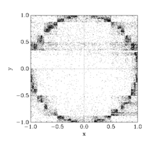
from the above illustration was integrated within a unit square using the suggested algorithm. The sampled points were recorded and plotted. Clearly stratified sampling algorithm concentrates the points in the regions where the variation of the function is largest.

Recursive stratified sampling is a generalization of one-dimensional adaptive quadratures to multi-dimensional integrals. On each recursion step the integral and the error are estimated using a plain Monte Carlo algorithm. If the error estimate is larger than the required accuracy the integration volume is divided into sub-volumes and the procedure is recursively applied to sub-volumes.

The ordinary 'dividing by two' strategy does not work for multi-dimensions as the number of sub-volumes grows far too quickly to keep track. Instead one estimates along which dimension a subdivision should bring the most dividends and only subdivides the volume along this dimension.

The stratified sampling algorithm concentrates the sampling points in the regions where the variance of the function is largest thus reducing the grand variance and making the sampling more effective, as shown on the illustration.

The popular MISER routine implements a similar algorithm.

MISER Monte Carlo

The MISER algorithm is based on recursive stratified sampling. This technique aims to reduce the overall integration error by concentrating integration points in the regions of highest variance.[7]

The idea of stratified sampling begins with the observation that for two disjoint regions a and b with Monte Carlo estimates of the integral ${\displaystyle E_{a}(f)}$ and ${\displaystyle E_{b}(f)}$ and variances ${\displaystyle \sigma _{a}^{2}(f)}$ and ${\displaystyle \sigma _{b}^{2}(f)}$, the variance Var(f) of the combined estimate

${\displaystyle E(f)={\tfrac {1}{2}}\left(E_{a}(f)+E_{b}(f)\right)}$

is given by,

${\displaystyle \mathrm {Var} (f)={\frac {\sigma _{a}^{2}(f)}{4N_{a}}}+{\frac {\sigma _{b}^{2}(f)}{4N_{b}}}}$

It can be shown that this variance is minimized by distributing the points such that,

${\displaystyle {\frac {N_{a}}{N_{a}+N_{b}}}={\frac {\sigma _{a}}{\sigma _{a}+\sigma _{b}}}}$

Hence the smallest error estimate is obtained by allocating sample points in proportion to the standard deviation of the function in each sub-region.

The MISER algorithm proceeds by bisecting the integration region along one coordinate axis to give two sub-regions at each step. The direction is chosen by examining all d possible bisections and selecting the one which will minimize the combined variance of the two sub-regions. The variance in the sub-regions is estimated by sampling with a fraction of the total number of points available to the current step. The same procedure is then repeated recursively for each of the two half-spaces from the best bisection. The remaining sample points are allocated to the sub-regions using the formula for N_a and N_b. This recursive allocation of integration points continues down to a user-specified depth where each sub-region is integrated using a plain Monte Carlo estimate. These individual values and their error estimates are then combined upwards to give an overall result and an estimate of its error.

Importance sampling

Main article: Importance sampling

There are a variety of importance sampling algorithms, such as

Importance sampling algorithm

Importance sampling provides a very important tool to perform Monte-Carlo integration.[3][8] The main result of importance sampling to this method is that the uniform sampling of ${\displaystyle {\overline {\mathbf {x} }}}$ is a particular case of a more generic choice, on which the samples are drawn from any distribution ${\displaystyle p({\overline {\mathbf {x} }})}$. The idea is that ${\displaystyle p({\overline {\mathbf {x} }})}$ can be chosen to decrease the variance of the measurement Q_N.

Consider the following example where one would like to numerically integrate a gaussian function, centered at 0, with σ = 1, from −1000 to 1000. Naturally, if the samples are drawn uniformly on the interval [−1000, 1000], only a very small part of them would be significant to the integral. This can be improved by choosing a different distribution from where the samples are chosen, for instance by sampling according to a gaussian distribution centered at 0, with σ = 1. Of course the "right" choice strongly depends on the integrand.

Formally, given a set of samples chosen from a distribution

${\displaystyle p({\overline {\mathbf {x} }}):\qquad {\overline {\mathbf {x} }}_{1},\cdots ,{\overline {\mathbf {x} }}_{N}\in V,}$

the estimator for I is given by[3]

${\displaystyle Q_{N}\equiv {\frac {1}{N}}\sum _{i=1}^{N}{\frac {f({\overline {\mathbf {x} }}_{i})}{p({\overline {\mathbf {x} }}_{i})}}}$

Intuitively, this says that if we pick a particular sample twice as much as other samples, we weight it half as much as the other samples. This estimator is naturally valid for uniform sampling, the case where ${\displaystyle p({\overline {\mathbf {x} }})}$ is constant.

The Metropolis-Hastings algorithm is one of the most used algorithms to generate ${\displaystyle {\overline {\mathbf {x} }}}$ from ${\displaystyle p({\overline {\mathbf {x} }})}$,[3] thus providing an efficient way of computing integrals.

Multiple and adaptive importance sampling

When different proposal distributions, ${\displaystyle p_{n}({\overline {\mathbf {x} }})}$ , ${\displaystyle n=1,\ldots ,N,}$ are jointly used for drawing the samples ${\displaystyle {\overline {\mathbf {x} }}_{1},\cdots ,{\overline {\mathbf {x} }}_{N}\in V,}$ different proper weighting functions can be employed (e.g., see [9][10][11]). In an adaptive setting, the proposal distributions, ${\displaystyle p_{n,t}({\overline {\mathbf {x} }})}$ , ${\displaystyle n=1,\ldots ,N,}$ and ${\displaystyle t=1,\ldots ,T,}$ are updated each iteration ${\displaystyle t}$ of the adaptive importance sampling algorithm. Hence, since a population of proposal densities is used, several suitable combinations of sampling and weighting schemes can be employed.[12][13][14][15][16]

VEGAS Monte Carlo

Main article: VEGAS algorithm

The VEGAS algorithm approximates the exact distribution by making a number of passes over the integration region which creates the histogram of the function f. Each histogram is used to define a sampling distribution for the next pass. Asymptotically this procedure converges to the desired distribution.[17] In order to avoid the number of histogram bins growing like K^d, the probability distribution is approximated by a separable function:

${\displaystyle g(x_{1},x_{2},\ldots )=g_{1}(x_{1})g_{2}(x_{2})\ldots }$

so that the number of bins required is only Kd. This is equivalent to locating the peaks of the function from the projections of the integrand onto the coordinate axes. The efficiency of VEGAS depends on the validity of this assumption. It is most efficient when the peaks of the integrand are well-localized. If an integrand can be rewritten in a form which is approximately separable this will increase the efficiency of integration with VEGAS. VEGAS incorporates a number of additional features, and combines both stratified sampling and importance sampling.[17]

See also

• Auxiliary field Monte Carlo
• Monte Carlo method in statistical physics
• Monte Carlo method
• Variance reduction

Notes

1. Press et al, 2007, Chap. 4.
2. Press et al, 2007, Chap. 7.
3. Newman, 1999, Chap. 2.
4. Newman, 1999, Chap. 1.
5. Press et al, 2007
6. MacKay, David (2003). "chapter 4.4 Typicality & chapter 29.1" (PDF). Information Theory, Inference and Learning Algorithms. Cambridge University Press. pp. 284–292. ISBN 978-0-521-64298-9. MR 2012999.
7. Press, 1990, pp 190-195.
8. Kroese, D. P.; Taimre, T.; Botev, Z. I. (2011). Handbook of Monte Carlo Methods. John Wiley & Sons.
9. Veach, Eric; Guibas, Leonidas J. (1995-01-01). Optimally Combining Sampling Techniques for Monte Carlo Rendering10.1145/218380.218498. Proceedings of the 22Nd Annual Conference on Computer Graphics and Interactive Techniques. SIGGRAPH '95. New York, NY, USA. pp. 419–428. CiteSeerX 10.1.1.127.8105. doi:10.1145/218380.218498. ISBN 978-0-89791-701-8.
10. Owen, Art; Associate, Yi Zhou (2000-03-01). "Safe and Effective Importance Sampling". Journal of the American Statistical Association. 95 (449): 135–143. CiteSeerX 10.1.1.36.4536. doi:10.1080/01621459.2000.10473909. ISSN 0162-1459.
11. Elvira, V.; Martino, L.; Luengo, D.; Bugallo, M.F. (2015-10-01). "Efficient Multiple Importance Sampling Estimators". IEEE Signal Processing Letters. 22 (10): 1757–1761. arXiv:1505.05391. Bibcode:2015ISPL...22.1757E. doi:10.1109/LSP.2015.2432078. ISSN 1070-9908.
12. Cappé, O.; Guillin, A.; Marin, J. M.; Robert, C. P. (2004-12-01). "Population Monte Carlo". Journal of Computational and Graphical Statistics. 13 (4): 907–929. doi:10.1198/106186004X12803. ISSN 1061-8600.
13. Cappé, Olivier; Douc, Randal; Guillin, Arnaud; Marin, Jean-Michel; Robert, Christian P. (2008-04-25). "Adaptive importance sampling in general mixture classes". Statistics and Computing. 18 (4): 447–459. arXiv:0710.4242. doi:10.1007/s11222-008-9059-x. ISSN 0960-3174.
14. Cornuet, Jean-Marie; Marin, Jean-Michel; Mira, Antonietta; Robert, Christian P. (2012-12-01). "Adaptive Multiple Importance Sampling". Scandinavian Journal of Statistics. 39 (4): 798–812. arXiv:0907.1254. doi:10.1111/j.1467-9469.2011.00756.x. ISSN 1467-9469.
15. Martino, L.; Elvira, V.; Luengo, D.; Corander, J. (2015-08-01). "An Adaptive Population Importance Sampler: Learning From Uncertainty". IEEE Transactions on Signal Processing. 63 (16): 4422–4437. Bibcode:2015ITSP...63.4422M. CiteSeerX 10.1.1.464.9395. doi:10.1109/TSP.2015.2440215. ISSN 1053-587X.
16. Bugallo, Mónica F.; Martino, Luca; Corander, Jukka (2015-12-01). "Adaptive importance sampling in signal processing". Digital Signal Processing. Special Issue in Honour of William J. (Bill) Fitzgerald. 47: 36–49. doi:10.1016/j.dsp.2015.05.014.
17. Lepage, 1978

References

• Caflisch, R. E. (1998). "Monte Carlo and quasi-Monte Carlo methods". Acta Numerica. 7: 1–49. Bibcode:1998AcNum...7....1C. doi:10.1017/S0962492900002804.
• Weinzierl, S. (2000). "Introduction to Monte Carlo methods". arXiv:hep-ph/0006269.
• Press, W. H.; Farrar, G. R. (1990). "Recursive Stratified Sampling for Multidimensional Monte Carlo Integration". Computers in Physics. 4 (2): 190. Bibcode:1990ComPh...4..190P. doi:10.1063/1.4822899.
• Lepage, G. P. (1978). "A New Algorithm for Adaptive Multidimensional Integration". Journal of Computational Physics. 27 (2): 192–203. Bibcode:1978JCoPh..27..192L. doi:10.1016/0021-9991(78)90004-9.
• Lepage, G. P. (1980). "VEGAS: An Adaptive Multi-dimensional Integration Program". Cornell Preprint CLNS 80-447.
• Hammersley, J. M.; Handscomb, D. C. (1964). Monte Carlo Methods. Methuen. ISBN 978-0-416-52340-9.
• Press, WH; Teukolsky, SA; Vetterling, WT; Flannery, BP (2007). Numerical Recipes: The Art of Scientific Computing (3rd ed.). New York: Cambridge University Press. ISBN 978-0-521-88068-8.
• Newman, MEJ; Barkema, GT (1999). Monte Carlo Methods in Statistical Physics. Clarendon Press.
• Robert, CP; Casella, G (2004). Monte Carlo Statistical Methods (2nd ed.). Springer. ISBN 978-1-4419-1939-7.

External links

• Café math : Monte Carlo Integration : A blog article describing Monte Carlo integration (principle, hypothesis, confidence interval)
• Boost.Math : Naive Monte Carlo integration: Documentation for the C++ naive Monte-Carlo routines
• Monte Carlo applet applied in statistical physics problems