Interpolation

In the mathematical field of numerical analysis, interpolation is a type of estimation, a method of constructing new data points within the range of a discrete set of known data points.[1]

For other uses, see Interpolation (disambiguation).

In engineering and science, one often has a number of data points, obtained by sampling or experimentation, which represent the values of a function for a limited number of values of the independent variable. It is often required to interpolate, i.e., estimate the value of that function for an intermediate value of the independent variable.

A closely related problem is the approximation of a complicated function by a simple function. Suppose the formula for some given function is known, but too complicated to evaluate efficiently. A few data points from the original function can be interpolated to produce a simpler function which is still fairly close to the original. The resulting gain in simplicity may outweigh the loss from interpolation error.

An interpolation of a finite set of points on an epitrochoid. The points in red are connected by blue interpolated spline curves deduced only from the red points. The interpolated curves have polynomial formulas much simpler than that of the original epitrochoid curve.

Example

This table gives some values of an unknown function ${\displaystyle f(x)}$.

Plot of the data points as given in the table.

	${\displaystyle x}$		${\displaystyle f(x)}$
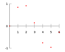
	0		0
	1		0	.	8415
	2		0	.	9093
	3		0	.	1411
	4		−0	.	7568
	5		−0	.	9589
	6		−0	.	2794

Interpolation provides a means of estimating the function at intermediate points, such as ${\displaystyle x=2.5}$.

We describe some methods of interpolation, differing in such properties as: accuracy, cost, number of data points needed, and smoothness of the resulting interpolant function.

Piecewise constant interpolation

Piecewise constant interpolation, or nearest-neighbor interpolation.

Further information: Nearest-neighbor interpolation

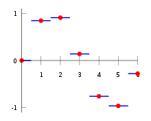
The simplest interpolation method is to locate the nearest data value, and assign the same value. In simple problems, this method is unlikely to be used, as linear interpolation (see below) is almost as easy, but in higher-dimensional multivariate interpolation, this could be a favourable choice for its speed and simplicity.

Linear interpolation

Plot of the data with linear interpolation superimposed

Main article: Linear interpolation

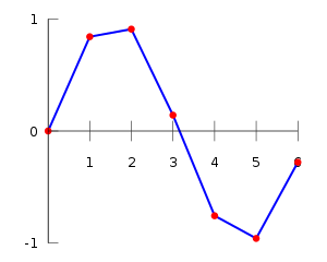
One of the simplest methods is linear interpolation (sometimes known as lerp). Consider the above example of estimating f(2.5). Since 2.5 is midway between 2 and 3, it is reasonable to take f(2.5) midway between f(2) = 0.9093 and f(3) = 0.1411, which yields 0.5252.

Generally, linear interpolation takes two data points, say (x_a,y_a) and (x_b,y_b), and the interpolant is given by:

${\displaystyle y=y_{a}+\left(y_{b}-y_{a}\right){\frac {x-x_{a}}{x_{b}-x_{a}}}{\text{ at the point }}\left(x,y\right)}$

${\displaystyle {\frac {y-y_{a}}{y_{b}-y_{a}}}={\frac {x-x_{a}}{x_{b}-x_{a}}}}$

${\displaystyle {\frac {y-y_{a}}{x-x_{a}}}={\frac {y_{b}-y_{a}}{x_{b}-x_{a}}}}$

This previous equation states that the slope of the new line between ${\displaystyle (x_{a},y_{a})}$ and ${\displaystyle (x,y)}$ is the same as the slope of the line between ${\displaystyle (x_{a},y_{a})}$ and ${\displaystyle (x_{b},y_{b})}$

Linear interpolation is quick and easy, but it is not very precise. Another disadvantage is that the interpolant is not differentiable at the point x_k.

The following error estimate shows that linear interpolation is not very precise. Denote the function which we want to interpolate by g, and suppose that x lies between x_a and x_b and that g is twice continuously differentiable. Then the linear interpolation error is

${\displaystyle |f(x)-g(x)|\leq C(x_{b}-x_{a})^{2}\quad {\text{where}}\quad C={\frac {1}{8}}\max _{r\in [x_{a},x_{b}]}|g''(r)|.}$

In words, the error is proportional to the square of the distance between the data points. The error in some other methods, including polynomial interpolation and spline interpolation (described below), is proportional to higher powers of the distance between the data points. These methods also produce smoother interpolants.

Polynomial interpolation

Plot of the data with polynomial interpolation applied

Main article: Polynomial interpolation

Polynomial interpolation is a generalization of linear interpolation. Note that the linear interpolant is a linear function. We now replace this interpolant with a polynomial of higher degree.

Consider again the problem given above. The following sixth degree polynomial goes through all the seven points:

${\displaystyle f(x)=-0.0001521x^{6}-0.003130x^{5}+0.07321x^{4}-0.3577x^{3}+0.2255x^{2}+0.9038x.}$

Substituting x = 2.5, we find that f(2.5) = 0.5965.

Generally, if we have n data points, there is exactly one polynomial of degree at most n−1 going through all the data points. The interpolation error is proportional to the distance between the data points to the power n. Furthermore, the interpolant is a polynomial and thus infinitely differentiable. So, we see that polynomial interpolation overcomes most of the problems of linear interpolation.

However, polynomial interpolation also has some disadvantages. Calculating the interpolating polynomial is computationally expensive (see computational complexity) compared to linear interpolation. Furthermore, polynomial interpolation may exhibit oscillatory artifacts, especially at the end points (see Runge's phenomenon).

Polynomial interpolation can estimate local maxima and minima that are outside the range of the samples, unlike linear interpolation. For example, the interpolant above has a local maximum at x ≈ 1.566, f(x) ≈ 1.003 and a local minimum at x ≈ 4.708, f(x) ≈ −1.003. However, these maxima and minima may exceed the theoretical range of the function—for example, a function that is always positive may have an interpolant with negative values, and whose inverse therefore contains false vertical asymptotes.

More generally, the shape of the resulting curve, especially for very high or low values of the independent variable, may be contrary to commonsense, i.e. to what is known about the experimental system which has generated the data points. These disadvantages can be reduced by using spline interpolation or restricting attention to Chebyshev polynomials.

Spline interpolation

Plot of the data with spline interpolation applied

Main article: Spline interpolation

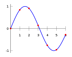
Remember that linear interpolation uses a linear function for each of intervals [x_k,x_k+1]. Spline interpolation uses low-degree polynomials in each of the intervals, and chooses the polynomial pieces such that they fit smoothly together. The resulting function is called a spline.

For instance, the natural cubic spline is piecewise cubic and twice continuously differentiable. Furthermore, its second derivative is zero at the end points. The natural cubic spline interpolating the points in the table above is given by

${\displaystyle f(x)={\begin{cases}-0.1522x^{3}+0.9937x,&{\text{if }}x\in [0,1],\\-0.01258x^{3}-0.4189x^{2}+1.4126x-0.1396,&{\text{if }}x\in [1,2],\\0.1403x^{3}-1.3359x^{2}+3.2467x-1.3623,&{\text{if }}x\in [2,3],\\0.1579x^{3}-1.4945x^{2}+3.7225x-1.8381,&{\text{if }}x\in [3,4],\\0.05375x^{3}-0.2450x^{2}-1.2756x+4.8259,&{\text{if }}x\in [4,5],\\-0.1871x^{3}+3.3673x^{2}-19.3370x+34.9282,&{\text{if }}x\in [5,6].\end{cases}}}$

In this case we get f(2.5) = 0.5972.

Like polynomial interpolation, spline interpolation incurs a smaller error than linear interpolation, while the interpolant is smoother and easier to evaluate than the high-degree polynomials used in polynomial interpolation. However, the global nature of the basis functions leads to ill-conditioning. This is completely mitigated by using splines of compact support, such as are implemented in Boost.Math and discussed in Kress.[2]

Function approximation

Interpolation is a common way to approximate functions. Given a function ${\displaystyle f:[a,b]\to \mathbb {R} }$ with a set of points ${\displaystyle x_{1},x_{2},\dots ,x_{n}\in [a,b]}$ one can form a function ${\displaystyle s:[a,b]\to \mathbb {R} }$ such that ${\displaystyle f(x_{i})=s(x_{i})}$ for ${\displaystyle i=1,2,\dots ,n}$ (that is that ${\displaystyle s}$ interpolates ${\displaystyle f}$ at these points). In general, an interpolant need not be a good approximation, but there are well known and often reasonable conditions where it will. For example, if ${\displaystyle f\in C^{4}([a,b])}$ (four times continuously differentiable) then cubic spline interpolation has an error bound given by ${\displaystyle \|f-s\|_{\infty }\leq C\|f^{(4)}\|_{\infty }h^{4}}$ where ${\displaystyle h\max _{i=1,2,\dots ,n-1}|x_{i+1}-x_{i}|}$ and ${\displaystyle C}$ is a constant.[3]

Via Gaussian processes

Gaussian process is a powerful non-linear interpolation tool. Many popular interpolation tools are actually equivalent to particular Gaussian processes. Gaussian processes can be used not only for fitting an interpolant that passes exactly through the given data points but also for regression, i.e., for fitting a curve through noisy data. In the geostatistics community Gaussian process regression is also known as Kriging.

Other forms

Other forms of interpolation can be constructed by picking a different class of interpolants. For instance, rational interpolation is interpolation by rational functions using Padé approximant, and trigonometric interpolation is interpolation by trigonometric polynomials using Fourier series. Another possibility is to use wavelets.

The Whittaker–Shannon interpolation formula can be used if the number of data points is infinite or if the function to be interpolated has compact support.

Sometimes, we know not only the value of the function that we want to interpolate, at some points, but also its derivative. This leads to Hermite interpolation problems.

When each data point is itself a function, it can be useful to see the interpolation problem as a partial advection problem between each data point. This idea leads to the displacement interpolation problem used in transportation theory.

In higher dimensions

Comparison of some 1- and 2-dimensional interpolations. Black and red/yellow/green/blue dots correspond to the interpolated point and neighbouring samples, respectively. Their heights above the ground correspond to their values.

Main article: Multivariate interpolation

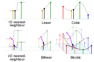
Multivariate interpolation is the interpolation of functions of more than one variable. Methods include bilinear interpolation and bicubic interpolation in two dimensions, and trilinear interpolation in three dimensions. They can be applied to gridded or scattered data.

• 
  Nearest neighbor
• 
  Bilinear
• 
  Bicubic

In digital signal processing

In the domain of digital signal processing, the term interpolation refers to the process of converting a sampled digital signal (such as a sampled audio signal) to that of a higher sampling rate (Upsampling) using various digital filtering techniques (e.g., convolution with a frequency-limited impulse signal). In this application there is a specific requirement that the harmonic content of the original signal be preserved without creating aliased harmonic content of the original signal above the original Nyquist limit of the signal (i.e., above fs/2 of the original signal sample rate). An early and fairly elementary discussion on this subject can be found in Rabiner and Crochiere's book Multirate Digital Signal Processing.[4]

Related concepts

The term extrapolation is used to find data points outside the range of known data points.

In curve fitting problems, the constraint that the interpolant has to go exactly through the data points is relaxed. It is only required to approach the data points as closely as possible (within some other constraints). This requires parameterizing the potential interpolants and having some way of measuring the error. In the simplest case this leads to least squares approximation.

Approximation theory studies how to find the best approximation to a given function by another function from some predetermined class, and how good this approximation is. This clearly yields a bound on how well the interpolant can approximate the unknown function.

Generalization

If we consider ${\displaystyle x}$ as a variable in a topological space, and the function ${\displaystyle f(x)}$ mapping to a Banach space, then the problem is treated as "interpolation of operators".[5] The classical results about interpolation of operators are the Riesz–Thorin theorem and the Marcinkiewicz theorem. There are also many other subsequent results.

See also

• Barycentric coordinates – for interpolating within on a triangle or tetrahedron
• Bilinear interpolation
• Brahmagupta's interpolation formula
• Extrapolation
• Fractal interpolation
• Imputation (statistics)
• Lagrange interpolation
• Missing data
• Multivariate interpolation
• Newton–Cotes formulas
• Polynomial interpolation
• Radial basis function interpolation
• Simple rational approximation

References

1. Sheppard, William Fleetwood (1911). "Interpolation" . In Chisholm, Hugh (ed.). Encyclopædia Britannica. 14 (11th ed.). Cambridge University Press. pp. 706–710.
2. Kress, Rainer (1998). Numerical Analysis.
3. Hall, Charles A.; Meyer, Weston W. (1976). "Optimal Error Bounds for Cubic Spline Interpolation". Journal of Approximation Theory. 16 (2): 105–122. doi:10.1016/0021-9045(76)90040-X.
4. R.E. Crochiere and L.R. Rabiner. (1983). Multirate Digital Signal Processing. Englewood Cliffs, NJ: Prentice–Hall.
5. Colin Bennett, Robert C. Sharpley, Interpolation of Operators, Academic Press 1988

External links

• Online tools for linear, quadratic, cubic spline, and polynomial interpolation with visualisation and JavaScript source code.
• Sol Tutorials - Interpolation Tricks
• Compactly Supported Cubic B-Spline interpolation in Boost.Math
• Barycentric rational interpolation in Boost.Math
• Interpolation via the Chebyshev transform in Boost.Math