Huber loss

In statistics, the Huber loss is a loss function used in robust regression, that is less sensitive to outliers in data than the squared error loss. A variant for classification is also sometimes used.

Definition

Huber loss (green, ${\displaystyle \delta =1}$) and squared error loss (blue) as a function of ${\displaystyle y-f(x)}$

The Huber loss function describes the penalty incurred by an estimation procedure f. Huber (1964) defines the loss function piecewise by[1]

${\displaystyle L_{\delta }(a)={\begin{cases}{\frac {1}{2}}{a^{2}}&{\text{for }}|a|\leq \delta ,\\\delta (|a|-{\frac {1}{2}}\delta ),&{\text{otherwise.}}\end{cases}}}$

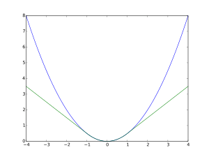
This function is quadratic for small values of a, and linear for large values, with equal values and slopes of the different sections at the two points where ${\displaystyle |a|=\delta }$. The variable a often refers to the residuals, that is to the difference between the observed and predicted values ${\displaystyle a=y-f(x)}$, so the former can be expanded to[2]

${\displaystyle L_{\delta }(y,f(x))={\begin{cases}{\frac {1}{2}}(y-f(x))^{2}&{\textrm {for}}|y-f(x)|\leq \delta ,\\\delta \,|y-f(x)|-{\frac {1}{2}}\delta ^{2}&{\textrm {otherwise.}}\end{cases}}}$

Motivation

Two very commonly used loss functions are the squared loss, ${\displaystyle L(a)=a^{2}}$, and the absolute loss, ${\displaystyle L(a)=|a|}$. The squared loss function results in an arithmetic mean-unbiased estimator, and the absolute-value loss function results in a median-unbiased estimator (in the one-dimensional case, and a geometric median-unbiased estimator for the multi-dimensional case). The squared loss has the disadvantage that it has the tendency to be dominated by outliers—when summing over a set of ${\displaystyle a}$'s (as in ${\textstyle \sum _{i=1}^{n}L(a_{i})}$), the sample mean is influenced too much by a few particularly large ${\displaystyle a}$-values when the distribution is heavy tailed: in terms of estimation theory, the asymptotic relative efficiency of the mean is poor for heavy-tailed distributions.

As defined above, the Huber loss function is strongly convex in a uniform neighborhood of its minimum ${\displaystyle a=0}$; at the boundary of this uniform neighborhood, the Huber loss function has a differentiable extension to an affine function at points ${\displaystyle a=-\delta }$ and ${\displaystyle a=\delta }$. These properties allow it to combine much of the sensitivity of the mean-unbiased, minimum-variance estimator of the mean (using the quadratic loss function) and the robustness of the median-unbiased estimator (using the absolute value function).

Pseudo-Huber loss function

The Pseudo-Huber loss function can be used as a smooth approximation of the Huber loss function. It combines the best properties of L2 squared loss and L1 absolute loss by being strongly convex when close to the target/minimum and less steep for extreme values. This steepness can be controlled by the ${\displaystyle \delta }$ value. The Pseudo-Huber loss function ensures that derivatives are continuous for all degrees. It is defined as[3][4]

${\displaystyle L_{\delta }(a)=\delta ^{2}\left({\sqrt {1+(a/\delta )^{2}}}-1\right).}$

As such, this function approximates ${\displaystyle a^{2}/2}$ for small values of ${\displaystyle a}$, and approximates a straight line with slope ${\displaystyle \delta }$ for large values of ${\displaystyle a}$.

While the above is the most common form, other smooth approximations of the Huber loss function also exist.[5]

Variant for classification

For classification purposes, a variant of the Huber loss called modified Huber is sometimes used. Given a prediction ${\displaystyle f(x)}$ (a real-valued classifier score) and a true binary class label ${\displaystyle y\in \{+1,-1\}}$, the modified Huber loss is defined as[6]

${\displaystyle L(y,f(x))={\begin{cases}\max(0,1-y\,f(x))^{2}&{\textrm {for}}\,\,y\,f(x)\geq -1,\\-4y\,f(x)&{\textrm {otherwise.}}\end{cases}}}$

The term ${\displaystyle \max(0,1-y\,f(x))}$ is the hinge loss used by support vector machines; the quadratically smoothed hinge loss is a generalization of ${\displaystyle L}$.[6]

Applications

The Huber loss function is used in robust statistics, M-estimation and additive modelling.[7]

See also

• Winsorizing
• Robust regression
• M-estimator
• Visual comparison of different M-estimators

References

1. Huber, Peter J. (1964). "Robust Estimation of a Location Parameter". Annals of Statistics. 53 (1): 73–101. doi:10.1214/aoms/1177703732. JSTOR 2238020.
2. Hastie, Trevor; Tibshirani, Robert; Friedman, Jerome (2009). The Elements of Statistical Learning. p. 349. Archived from the original on 2015-01-26. Compared to Hastie et al., the loss is scaled by a factor of ½, to be consistent with Huber's original definition given earlier.
3. Charbonnier, P.; Blanc-Feraud, L.; Aubert, G.; Barlaud, M. (1997). "Deterministic edge-preserving regularization in computed imaging". IEEE Trans. Image Processing. 6 (2): 298–311. CiteSeerX 10.1.1.64.7521. doi:10.1109/83.551699. PMID 18282924.
4. Hartley, R.; Zisserman, A. (2003). Multiple View Geometry in Computer Vision (2nd ed.). Cambridge University Press. p. 619. ISBN 978-0-521-54051-3.
5. Lange, K. (1990). "Convergence of Image Reconstruction Algorithms with Gibbs Smoothing". IEEE Trans. Med. Imaging. 9 (4): 439–446. doi:10.1109/42.61759. PMID 18222791.
6. Zhang, Tong (2004). Solving large scale linear prediction problems using stochastic gradient descent algorithms. ICML.
7. Friedman, J. H. (2001). "Greedy Function Approximation: A Gradient Boosting Machine". Annals of Statistics. 26 (5): 1189–1232. doi:10.1214/aos/1013203451. JSTOR 2699986.