Hosmer–Lemeshow test

The Hosmer–Lemeshow test is a statistical test for goodness of fit for logistic regression models. It is used frequently in risk prediction models. The test assesses whether or not the observed event rates match expected event rates in subgroups of the model population. The Hosmer–Lemeshow test specifically identifies subgroups as the deciles of fitted risk values. Models for which expected and observed event rates in subgroups are similar are called well calibrated.

Introduction

Motivation

Logistic regression models provide an estimate of the probability of an outcome, usually designated as a "success". It is desirable that the estimated probability of success be close to the true probability. Consider the following example.

A researcher wishes to know if caffeine improves performance on a memory test. Volunteers consume different amounts of caffeine from 0 to 500 mg, and their score on the memory test is recorded. The results are shown in the table below.

group	caffeine	n.volunteers	A.grade	proportion.A
1	0	30	10	0.33
2	50	30	13	0.43
3	100	30	17	0.57
4	150	30	15	0.50
5	200	30	10	0.33
6	250	30	5	0.17
7	300	30	4	0.13
8	350	30	3	0.10
9	400	30	3	0.10
10	450	30	1	0.03
11	500	30	0	0

The table has the following columns.

group: identifier for the 11 treatment groups, each receiving a different dose
caffeine: mg of caffeine for volunteers in a treatment group
n.volunteers: number of volunteers in a treatment group
A.grade: the number of volunteers who achieved an A grade in the memory test (success)
proportion.A: the proportion of volunteers who achieved an A grade

The researcher performs a logistic regression, where "success" is a grade of A in the memory test, and the explanatory (x) variable is dose of caffeine. The logistic regression indicates that caffeine dose is significantly associated with the probability of an A grade (p < 0.001). However, the plot of the probability of an A grade versus mg caffeine shows that the logistic model (red line) does not accurately predict the probability seen in the data (black circles).

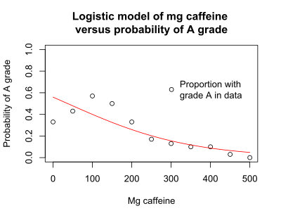
The logistic model suggests that the highest proportion of A scores will occur in volunteers who consume zero mg caffeine, when in fact the highest proportion of A scores occurs in volunteer consuming in the range of 100 to 150 mg.

The same information may be presented in another graph that is helpful when there are two or more explanatory (x) variables. This is a graph of observed proportion of successes in the data and the expected proportion as predicted by the logistic model. Ideally all the points fall on the diagonal red line.

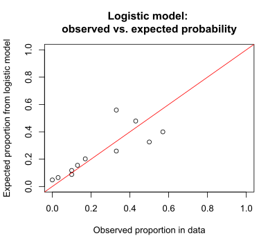
The expected probability of success (a grade of A) is given by the equation for the logistic regression model:

p(success)={\frac {1}{1+e^{-(b_{0}+b_{1}x_{1})}}}

where b₀ and b₁ are specified by the logistic regression model:

b₀ is the intercept
b₁ is the coefficient for x₁

For the logistic model of P(success) vs dose of caffeine, both graphs show that, for many doses, the estimated probability is not close to the probability observed in the data. This occurs even though the regression gave a significant p-value for caffeine. It is possible to have a significant p-value, but still have poor predictions of the proportion of successes. The Hosmer–Lemeshow test is useful to determine if the poor predictions (lack of fit) are significant, indicating that there are problems with the model.

There are many possible reasons that a model may give poor predictions. In this example, the plot of the logistic regression suggests that the probability of an A score does not change monotonically with caffeine dose, as assumed by the model. Instead, it increases (from 0 to 100 mg) and then decreases. The current model is P(success) vs caffeine, and appears to be an inadequate model. A better model might be P(success) vs caffeine + caffeine^2. The addition of the quadratic term caffeine^2 to the regression model would allow for the increasing and then decreasing relationship of grade to caffeine dose. The logistic model including the caffeine^2 term indicates that the quadratic caffeine^2 term is significant (p=0.003) while the linear caffeine term is not significant (p=0.21).

The graph below shows the observed proportion of successes in the data versus the expected proportion as predicted by the logistic model that includes the caffeine^2 term.

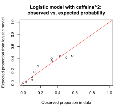
The Hosmer–Lemeshow test can determine if the differences between observed and expected proportions are significant, indicating model lack of fit.

Pearson chi-squared goodness of fit test

The Pearson chi-squared goodness of fit test provides a method to test if the observed and expected proportions differ significantly. This method is useful if there are many observations for each value of the x variable(s).

For the caffeine example, the observed number of A grades and non-A grades are known. The expected number (from the logistic model) can be calculated using the equation from the logistic regression. These are shown in the table below.

The null hypothesis is that the observed and expected proportions are the same across all doses. The alternative hypothesis is that the observed and expected proportions are not the same.

The Pearson chi-squared statistic is the sum of (observed – expected)^2/expected. For the caffeine data, the Pearson chi-squared statistic is 17.46. The number of degrees of freedom is the number of doses (11) minus the number of parameters from the logistic regression (2), giving 11 - 2 = 9 degrees of freedom. The probability that a chi-square statistic with df=9 will be 17.46 or greater is p = 0.042. This result indicates that, for the caffeine example, the observed and expected proportions of A grades differ significantly. The model does not accurately predict the probability of an A grade, given the caffeine dose. This result is consistent with the graphs above.

In this caffeine example, there are 30 observations for each dose, which makes calculation of the Pearson chi-squared statistic feasible. Unfortunately, it is common that there are not enough observations for each possible combinations of values of the x variables, so the Pearson chi-squared statistic cannot be readily calculated. A solution to this problem is the Hosmer-Lemeshow statistic. The key concept of the Hosmer-Lemeshow statistic is that, instead of observations being grouped by the values of the x variable(s), the observations are grouped by expected probability. That is, observations with similar expected probability are put into the same group, usually to create approximately 10 groups.

Calculation of the statistic

The Hosmer–Lemeshow test statistic is given by:

H=\sum _{g=1}^{G}\left({\frac {(O_{1g}-E_{1g})^{2}}{E_{1g}}}+{\frac {(O_{0g}-E_{0g})^{2}}{E_{0g}}}\right)=\sum _{g=1}^{G}\left({\frac {(O_{1g}-E_{1g})^{2}}{N_{g}\pi _{g}}}+{\frac {(N_{g}-O_{1g}-(N_{g}-E_{1g}))^{2}}{N_{g}(1-\pi _{g})}}\right)=\sum _{g=1}^{G}{\frac {(O_{1g}-E_{1g})^{2}}{N_{g}\pi _{g}(1-\pi _{g})}}.\,\!

Here O_1g, E_1g, O_0g, E_0g, N_g, and π_g denote the observed Y=1 events, expected Y=1 events, observed Y=0 events, expected Y=0 events, total observations, predicted risk for the g^th risk decile group, and G is the number of groups. The test statistic asymptotically follows a $\chi ^{2}$ distribution with G − 2 degrees of freedom. The number of risk groups may be adjusted depending on how many fitted risks are determined by the model. This helps to avoid singular decile groups.

The Pearson chi-squared goodness of fit test cannot be readily applied if there are only one or a few observations for each possible value of an x variable, or for each possible combination of values of x variables. The Hosmer-Lemeshow statistic was developed to address this problem.

Suppose that, in the caffeine study, the researcher was not able to assign 30 volunteers to each dose. Instead, 170 volunteers reported the estimated amount of caffeine they consumed in the previous 24 hours. The data are shown in the table below.

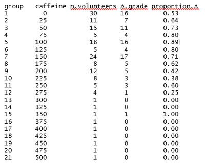
The table shows that, for many dose levels, there are only one or a few observations. The Pearson chi-squared statistic would not give reliable estimates in this situation.

The logistic regression model for the caffeine data for 170 volunteers indicates that caffeine dose is significantly associated with an A grade, p < 0.001. The graph shows that there is a downward slope. However, the probability of an A grade as predicted by the logistic model (red line) does not accurately predict the probability estimated from the data for each dose (black circles). Despite the significant p-value for caffeine dose, there is lack of fit of the logistic curve to the observed data.

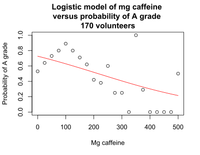
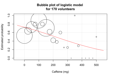
This version of the graph can be somewhat misleading, because different numbers of volunteers take each dose. In an alternative graph, the bubble plot, the size of the circle is proportional to the number of volunteers.[1]

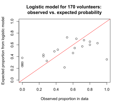
The plot of observed versus expected probability also indicates the lack of fit of the model, with much scatter around the ideal diagonal.

Calculation of the Hosmer-Lemeshow statistic proceeds in 6 steps,[2] using the caffeine data for 170 volunteers as an example.

1. Compute p(success) for all n subjects

Compute p(success) for each subject using the coefficients from the logistic regression. Subjects with the same values for the explanatory variables will have the same estimated probability of success. The table below shows the p(success), the expected proportion of volunteers with an A grade, as predicted by the logistic model.

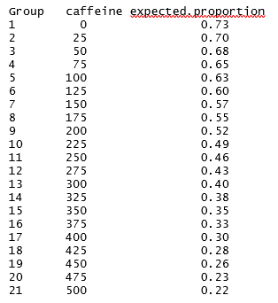
2. Order p(success) from largest to smallest values

The table from Step 1 is sorted by p(success), the expected proportion. If every volunteer took a different dose, there would be 170 different values in the table. Because there are only 21 unique dose values, there are only 21 unique values of p(success).

3. Divide the ordered values into Q percentile groups

The ordered values of p(success) are divided into Q groups. The number of groups, Q, is typically 10. Because of tied values for p(success), the number of subjects in each group may not be identical. Different software implementations of the Hosmer–Lemeshow test use different methods for handling subjects with the same p(success), so the cut points to create the Q groups may differ. In addition, using a different value for Q will produce different cut points. The table in Step 4 shows the Q = 10 intervals for the caffeine data.

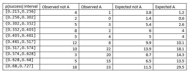
4. Create a table of observed and expected counts

The observed number of successes and failures in each interval are obtained by counting the subjects in that interval. The expected number of successes in an interval is the sum of the probability of success for the subjects in that interval.

The table below shows the cut points for the p(success) intervals selected by the R function HLTest() from Bilder and Loughin, with the number of observed and expected A and not A.

5. Calculate the Hosmer-Lemeshow statistic from the table

The Hosmer-Lemeshow statistic is calculated using the formula given in the introduction, which for the caffeine example is 17.103.

H=\sum _{q=1}^{10}\left({\frac {(Observed.A-Expected.A)^{2}}{Expected.A}}+{\frac {(Observed.not.A-Expected.not.A)^{2}}{Expected.not.A}}\right)

6. Calculate the p-value

Compare the computed Hosmer-Lemeshow statistic to a chi-squared distribution with Q-2 degrees of freedom to calculate the p-value.

There are Q = 10 groups in the caffeine example, giving 10 – 2 = 8 degrees of freedom. The p-value for a chi-squared statistic of 17.103 with df = 8 is p = 0.029. The p-value is below alpha = 0.05, so the null hypothesis that the observed and expected proportions are the same across all doses is rejected. The way to compute this is to get a cumulative distribution function for a right-tail chi-square distribution with 8 degrees of freedom, i.e. cdf_chisq_rt(x, 8), or 1-cdf_chisq_lt(x, 8).

Limitations and alternatives

The Hosmer–Lemeshow test has limitations. Harrell describes several:[3]

"The Hosmer-Lemeshow test is for overall calibration error, not for any particular lack of fit such as quadratic effects. It does not properly take overfitting into account, is arbitrary to choice of bins and method of computing quantiles, and often has power that is too low."

"For these reasons the Hosmer-Lemeshow test is no longer recommended. Hosmer et al have a better one d.f. omnibus test of fit, implemented in the R rms package residuals.lrm function."

"But I recommend specifying the model to make it more likely to fit up front (especially with regard to relaxing linearity assumptions using regression splines) and using the bootstrap to estimate overfitting and to get an overfitting-corrected high-resolution smooth calibration curve to check absolute accuracy. These are done using the R rms package."

Other alternatives have been developed to address the limitations of the Hosmer-Lemeshow test. These include the Osius-Rojek test and the Stukel test.[4]

gollark: No, the new one.

gollark: Oh, did you read the latest antimemetics division™ update?

gollark: ↑←

gollark: ↑

gollark: What if BF but also bee movie script?

References

Bilder, Christopher R.; Loughin, Thomas M. (2014), Analysis of Categorical Data with R (First ed.), Chapman and Hall/CRC, ISBN 978-1439855676
Kleinbaum, David G.; Klein, Mitchel (2012), Survival analysis: A Self-learning text (Third ed.), Springer, ISBN 978-1441966452
"r - Evaluating logistic regression and interpretation of Hosmer-Lemeshow Goodness of Fit". Cross Validated. Retrieved 2020-02-29.
available in the R script AllGOFTests.R: www.chrisbilder.com/categorical/Chapter5/AllGOFTests.R.

External links

Hosmer, David W.; Lemeshow, Stanley (2013). Applied Logistic Regression. New York: Wiley. ISBN 978-0-470-58247-3.
Alan Agresti (2012). Categorical Data Analysis. Hoboken: John Wiley and Sons. ISBN 978-0-470-46363-5.

This article is issued from Wikipedia. The text is licensed under Creative Commons - Attribution - Sharealike. Additional terms may apply for the media files.

[BilderLoughin2015-1] Bilder, Christopher R.; Loughin, Thomas M. (2014), Analysis of Categorical Data with R (First ed.), Chapman and Hall/CRC, ISBN 978-1439855676

[KleinbaumKlein2012-2] Kleinbaum, David G.; Klein, Mitchel (2012), Survival analysis: A Self-learning text (Third ed.), Springer, ISBN 978-1441966452

[3] "r - Evaluating logistic regression and interpretation of Hosmer-Lemeshow Goodness of Fit". Cross Validated. Retrieved 2020-02-29.

[4] vailable in the R script AllGOFTests.R: www.chrisbilder.com/categorical/Chapter5/AllGOFTests.R.