Hessian automatic differentiation
In applied mathematics, Hessian automatic differentiation are techniques based on automatic differentiation (AD) that calculate the second derivative of an -dimensional function, known as the Hessian matrix.
When examining a function in a neighborhood of a point, one can discard many complicated global aspects of the function and accurately approximate it with simpler functions. The quadratic approximation is the best-fitting quadratic in the neighborhood of a point, and is frequently used in engineering and science. To calculate the quadratic approximation, one must first calculate its gradient and Hessian matrix.
Let , for each the Hessian matrix is the second order derivative and is a symmetric matrix.
Reverse Hessian-vector products
For a given , this method efficiently calculates the Hessian-vector product . Thus can be used to calculate the entire Hessian by calculating , for .[1]
The method works by first using forward AD to perform , subsequently the method then calculates the gradient of using Reverse AD to yield . Both of these two steps come at a time cost proportional to evaluating the function, thus the entire Hessian can be evaluated at a cost proportional to n evaluations of the function.
Reverse Hessian: Edge_Pushing
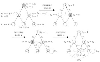
An algorithm that calculates the entire Hessian with one forward and one reverse sweep of the computational graph is Edge_Pushing. Edge_Pushing is the result of applying the reverse gradient to the computational graph of the gradient. Naturally, this graph has n output nodes, thus in a sense one has to apply the reverse gradient method to each outgoing node. Edge_Pushing does this by taking into account overlapping calculations.[2]

The algorithm's input is the computational graph of the function. After a preceding forward sweep where all intermediate values in the computational graph are calculated, the algorithm initiates a reverse sweep of the graph. Upon encountering a node that has a corresponding nonlinear elemental function, a new nonlinear edge is created between the node's predecessors indicating there is nonlinear interaction between them. See the example figure on the right. Appended to this nonlinear edge is an edge weight that is the second-order partial derivative of the nonlinear node in relation to its predecessors. This nonlinear edge is subsequently pushed down to further predecessors in such a way that when it reaches the independent nodes, its edge weight is the second-order partial derivative of the two independent nodes it connects.[2]
Graph colouring techniques for Hessians
The graph colouring techniques explore sparsity patterns of the Hessian matrix and cheap Hessian vector products to obtain the entire matrix. Thus these techniques are suited for large, sparse matrices. The general strategy of any such colouring technique is as follows.
- Obtain the global sparsity pattern of
- Apply a graph colouring algorithm that allows us to compact the sparsity structure.
- For each desired point calculate numeric entries of the compact matrix.
- Recover the Hessian matrix from the compact matrix.
Steps one and two need only be carried out once, and tend to be costly. When one wants to calculate the Hessian at numerous points (such as in an optimization routine), steps 3 and 4 are repeated.
 Coloured Sparsity pattern of the Hessian Matrix |
 The compact Hessian matrix |
As an example, the figure on the left shows the sparsity pattern of the Hessian matrix where the columns have been appropriately coloured in such a way to allow columns of the same colour to be merged without incurring in a collision between elements.
There are a number of colouring techniques, each with a specific recovery technique. For a comprehensive survey, see.[3] There have been successful numerical results of such methods.[4]
References
- Bruce Christianson. Automatic Hessians by Reverse Accumulation, http://imajna.oxfordjournals.org/content/12/2/135.abstract.
- R. Gower, M. Mello. A new framework for the computation of Hessians. In: Optimization Methods and Software. doi: http://www.tandfonline.com/doi/full/10.1080/10556788.2011.580098.
- A. H. Gebremedhin, A. Tarafdar, A. Pothen, and A. Walther. Efficient Computation of Sparse Hessians Using Coloring and Automatic Differentiation". In: INFORMS J. on Computing 21.2 (2009), pp. 209-223. doi:10.1287/ijoc.1080.0286
- A. Walther. Computing sparse Hessians with automatic differentiation". In: ACM Trans. Math. Softw. 34.1 (2008), pp. 1-15. ISSN 0098-3500. doi: http://doi.acm.org/10.1145/1322436.1322439.