Expansion path
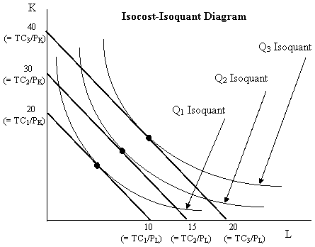
In economics, an expansion path (also called a scale line[1]) is a curve in a graph with quantities of two inputs, typically physical capital and labor, plotted on the axes. The path connects optimal input combinations as the scale of production expands.[2] A producer seeking to produce a given number of units of a product in the cheapest possible way chooses the point on the expansion path that is also on the isoquant associated with that output level.[3]

Economists Alfred Stonier and Douglas Hague defined “expansion path” as "that line which reflects the least–cost method of producing different levels of output, when factor prices remain constant."[4] The points on an expansion path occur where the firm's isocost curves, each showing fixed total input cost, and its isoquants, each showing a particular level of output, are tangent; each tangency point determines the firm's conditional factor demands. As a producer's level of output increases, the firm moves from one of these tangency points to the next; the curve joining the tangency points is called the expansion path.[5]
If an expansion path forms a straight line from the origin, the production technology is considered homothetic (or homoethetic).[6] In this case, the ratio of input usages is always the same regardless of the level of output, and the inputs can be expanded proportionately so as to maintain this optimal ratio as the level of output expands. A Cobb–Douglas production function is an example of a production function that has an expansion path which is a straight line through the origin.[6]
See also
- Income-consumption curve, the closest analog in consumer theory
References
- Jain, TR; Khanna OP (2008). Economics. VK Publications, ISBN 978-81-87344-77-3
- Hirschey, Mark (2008). Managerial economics. Cengage Learning, ISBN 978-0-324-58886-6
- Prusty, Sadananda (2010). Managerial Economics. PHI Learning Pvt. Ltd., ISBN 978-81-203-4094-7
- Stonier, Alfred W.; Hague, Douglas C. (1980). A textbook of economic theory, 5th edition. Longmans ISBN 978-0-582-29530-8
- Salvatore, Dominick (1989). Schaum's outline of theory and problems of managerial economics. McGraw-Hill, ISBN 978-0-07-054513-7
- Rasmussen, Svend (2011). Production Economics: The Basic Theory of Production Optimisation. Springer, ISBN 978-3-642-14609-1