Dynamic mode decomposition

Dynamic mode decomposition (DMD) is a dimensionality reduction algorithm developed by Peter Schmid in 2008. Given a time series of data, DMD computes a set of modes each of which is associated with a fixed oscillation frequency and decay/growth rate. For linear systems in particular, these modes and frequencies are analogous to the normal modes of the system, but more generally, they are approximations of the modes and eigenvalues of the composition operator (also called the Koopman operator). Due to the intrinsic temporal behaviors associated with each mode, DMD differs from dimensionality reduction methods such as principal component analysis, which computes orthogonal modes that lack predetermined temporal behaviors. Because its modes are not orthogonal, DMD-based representations can be less parsimonious than those generated by PCA. However, they can also be more physically meaningful because each mode is associated with a damped (or driven) sinusoidal behavior in time.

Overview

Dynamic mode decomposition was first introduced by Schmid as a numerical procedure for extracting dynamical features from flow data.[1]

The data takes the form of a snapshot sequence

${\displaystyle V_{1}^{N}=\{v_{1},v_{2},\dots ,v_{N}\},}$

where ${\displaystyle v_{i}\in \mathbb {R} ^{M}}$ is the ${\displaystyle i}$-th snapshot of the flow field, and ${\displaystyle V_{1}^{N}\in \mathbb {R} ^{M\times N}}$ is a data matrix whose columns are the individual snapshots. The subscript and superscript denote the index of the snapshot in the first and last columns respectively. These snapshots are assumed to be related via a linear mapping that defines a linear dynamical system

${\displaystyle v_{i+1}=Av_{i},}$

that remains approximately the same over the duration of the sampling period. Written in matrix form, this implies that

${\displaystyle V_{2}^{N}=AV_{1}^{N-1}+re_{N-1}^{T},}$

where ${\displaystyle r}$ is the vector of residuals that accounts for behaviors that cannot be described completely by ${\displaystyle A}$, ${\displaystyle e_{N-1}=\{0,0,\ldots ,1\}\in \mathbb {R} ^{N-1}}$, ${\displaystyle V_{1}^{N-1}=\{v_{1},v_{2},\dots ,v_{N-1}\}}$, and ${\displaystyle V_{2}^{N}=\{v_{2},v_{3},\dots ,v_{N}\}}$. Regardless of the approach, the output of DMD is the eigenvalues and eigenvectors of ${\displaystyle A}$, which are referred to as the DMD eigenvalues and DMD modes respectively.

Algorithm

There are two methods for obtaining these eigenvalues and modes. The first is Arnoldi-like, which is useful for theoretical analysis due to its connection with Krylov methods. The second is a singular value decomposition (SVD) based approach that is more robust to noise in the data and to numerical errors.

The Arnoldi approach

In fluids applications, the size of a snapshot, ${\displaystyle M}$, is assumed to be much larger than the number of snapshots ${\displaystyle N}$, so there are many equally valid choices of ${\displaystyle A}$. The original DMD algorithm picks ${\displaystyle A}$ so that each of the snapshots in ${\displaystyle V_{2}^{N}}$ can be written as the linear combination of the snapshots in ${\displaystyle V_{1}^{N-1}}$. Because most of the snapshots appear in both data sets, this representation is error free for all snapshots except ${\displaystyle v_{N}}$, which is written as

${\displaystyle v_{N}=a_{1}v_{1}+a_{2}v_{2}+\dots +a_{N-1}v_{N-1}+r=V_{1}^{N-1}a+r,}$

where ${\displaystyle a={a_{1},a_{2},\dots ,a_{N-1}}}$ is a set of coefficients DMD must identify and ${\displaystyle r}$ is the residual. In total,

${\displaystyle V_{2}^{N}=AV_{1}^{N-1}=V_{1}^{N-1}S+re_{N-1}^{T},}$

where ${\displaystyle S}$ is the companion matrix

${\displaystyle S={\begin{pmatrix}0&0&\dots &0&a_{1}\\1&0&\dots &0&a_{2}\\0&1&\dots &0&a_{3}\\\vdots &\vdots &\ddots &\vdots &\vdots \\0&0&\dots &1&a_{N-1}\end{pmatrix}}.}$

The vector ${\displaystyle a}$ can be computed by solving a least squares problem, which minimizes the overall residual. In particular if we take the QR decomposition of ${\displaystyle V_{1}^{N-1}=QR}$, then ${\displaystyle a=R^{-1}Q^{T}v_{N}}$.

In this form, DMD is a type of Arnoldi method, and therefore the eigenvalues of ${\displaystyle S}$ are approximations of the eigenvalues of ${\displaystyle A}$. Furthermore, if ${\displaystyle y}$ is an eigenvector of ${\displaystyle S}$, then ${\displaystyle V_{1}^{N-1}y}$ is an approximate eigenvector of ${\displaystyle A}$. The reason an eigendecomposition is performed on ${\displaystyle S}$ rather than ${\displaystyle A}$ is because ${\displaystyle S}$ is much smaller than ${\displaystyle A}$, so the computational cost of DMD is determined by the number of snapshots rather than the size of a snapshot.

The SVD-based approach

Instead of computing the companion matrix ${\displaystyle S}$, the SVD-based approach yields the matrix ${\displaystyle {\tilde {S}}}$ that is related to ${\displaystyle A}$ via a similarity transform. To do this, assume we have the SVD of ${\displaystyle V_{1}^{N-1}=U\Sigma W^{T}}$. Then

${\displaystyle V_{2}^{N}=AV_{1}^{N-1}+re_{N-1}^{T}=AU\Sigma W^{T}+re_{N-1}^{T}.}$

Equivalent to the assumption made by the Arnoldi-based approach, we choose ${\displaystyle A}$ such that the snapshots in ${\displaystyle V_{2}^{N}}$ can be written as the linear superposition of the columns in ${\displaystyle U}$, which is equivalent to requiring that they can be written as the superposition of POD modes. With this restriction, minimizing the residual requires that it is orthogonal to the POD basis (i.e., ${\displaystyle U^{T}r=0}$). Then multiplying both sides of the equation above by ${\displaystyle U^{T}}$ yields ${\displaystyle U^{T}V_{2}^{N}=U^{T}AU\Sigma W^{T}}$, which can be manipulated to obtain

${\displaystyle U^{T}AU=U^{T}V_{2}^{N}W\Sigma ^{-1}\equiv {\tilde {S}}.}$

Because ${\displaystyle A}$ and ${\displaystyle {\tilde {S}}}$ are related via similarity transform, the eigenvalues of ${\displaystyle S}$ are the eigenvalues of ${\displaystyle A}$, and if ${\displaystyle y}$ is an eigenvector of ${\displaystyle {\tilde {S}}}$, then ${\displaystyle Uy}$ is an eigenvector of ${\displaystyle A}$.

In summary, the SVD-based approach is as follows:

1. Split the time series of data in ${\displaystyle V_{1}^{N}}$ into the two matrices ${\displaystyle V_{1}^{N-1}}$ and ${\displaystyle V_{2}^{N}}$.
2. Compute the SVD of ${\displaystyle V_{1}^{N-1}=U\Sigma W^{T}}$.
3. Form the matrix ${\displaystyle {\tilde {S}}=U^{T}V_{2}^{N}W\Sigma ^{-1}}$, and compute its eigenvalues ${\displaystyle \lambda _{i}}$ and eigenvectors ${\displaystyle y_{i}}$.
4. The ${\displaystyle i}$-th DMD eigenvalues is ${\displaystyle \lambda _{i}}$ and ${\displaystyle i}$-th DMD mode is the ${\displaystyle Uy_{i}}$.

The advantage of the SVD-based approach over the Arnoldi-like approach is that noise in the data and numerical truncation issues can be compensated for by truncating the SVD of ${\displaystyle V_{1}^{N-1}}$. As noted in [1] accurately computing more than the first couple modes and eigenvalues can be difficult on experimental data sets without this truncation step.

Theoretical and algorithmic advancements

Since its inception in 2010, a considerable amount of work has focused on understanding and improving DMD. One of the first analyses of DMD by Rowley et al.[2] established the connection between DMD and the Koopman operator, and helped to explain the output of DMD when applied to nonlinear systems. Since then, a number of modifications have been developed that either strengthen this connection further or enhance the robustness and applicability of the approach.

• Optimized DMD: Optimized DMD is a modification of the original DMD algorithm designed to compensate for two limitations of that approach: (i) the difficulty of DMD mode selection, and (ii) the sensitivity of DMD to noise or other errors in the last snapshot of the time series.[3] Optimized DMD recasts the DMD procedure as an optimization problem where the identified linear operator has a fixed rank. Furthermore, unlike DMD which perfectly reproduces all of the snapshots except for the last, Optimized DMD allows the reconstruction errors to be distributed throughout the data set, which appears to make the approach more robust in practice.
• Optimal Mode Decomposition: Optimal Mode Decomposition (OMD) recasts the DMD procedure as an optimization problem and allows the user to directly impose the rank of the identified system.[4] Provided this rank is chosen properly, OMD can produce linear models with smaller residual errors and more accurate eigenvalues on both synthetic and experimental data sets.
• Exact DMD: The Exact DMD algorithm generalizes the original DMD algorithm in two ways. First, in the original DMD algorithm the data must be a time series of snapshots, but Exact DMD accepts a data set of snapshot pairs.[5] The snapshots in the pair must be separated by a fixed ${\displaystyle \Delta t}$, but do not need to be drawn from a single time series. In particular, Exact DMD can allow data from multiple experiments to be aggregated into a single data set. Second, the original DMD algorithm effectively pre-processes the data by projecting onto a set of POD modes. The Exact DMD algorithm removes this pre-processing step, and can produce DMD modes that cannot be written as the superposition of POD modes.
• Sparsity Promoting DMD: Sparsity promoting DMD is a post processing procedure for DMD mode and eigenvalue selection.[6] Sparsity promoting DMD uses an ${\displaystyle \ell _{1}}$ penalty to identify a smaller set of important DMD modes, and is an alternative approach to the DMD mode selection problem that can be solved efficiently using convex optimization techniques.
• Multi-Resolution DMD: Multi-Resolution DMD (mrDMD) is a combination of the techniques used in multiresolution analysis with Exact DMD designed to robust extracting DMD modes and eigenvalues from data sets containing multiple timescales.[7] The mrDMD approach was applied to global surface temperature data, and identifies a DMD mode that appears during El Nino years.
• Extended DMD: Extended DMD is a modification of Exact DMD that strengthens the connection between DMD and the Koopman operator.[8] As the name implies, Extended DMD is an extension of DMD that uses a richer set of observable functions to produce more accurate approximations of the Koopman operator. It also demonstrated the DMD and related methods produce approximations of the Koopman eigenfunctions in addition to the more commonly used eigenvalues and modes.
• DMD with Control: Dynamic mode decomposition with control (DMDc) [9] is a modification of the DMD procedure designed for data obtained from input output systems. One unique feature of DMDc is the ability to disambiguate the effects of system actuation from the open loop dynamics, which is useful when data are obtained in the presence of actuation.
• Total Least Squares DMD: Total Least Squares DMD is a recent modification of Exact DMD meant to address issues of robustness to measurement noise in the data. In,[10] the authors interpret the Exact DMD as a regression problem that is solved using ordinary least squares (OLS), which assumes that the regressors are noise free. This assumption creates a bias in the DMD eigenvalues when it is applied to experimental data sets where all of the observations are noisy. Total least squares DMD replaces the OLS problem with a total least squares problem, which eliminates this bias.
• Dynamic Distribution Decomposition: DDD focuses on the forward problem in continuous time, i.e., the transfer operator. However the method developed can also be used for fitting DMD problems in continuous time [11].

In addition to the algorithms listed here, similar application-specific techniques have been developed. For example, like DMD, Prony's method represents a signal as the superposition of damped sinusoids. In climate science, linear inverse modeling is also strongly connected with DMD.[12] For a more comprehensive list, see Tu et al.[5]

Examples

Trailing edge of a profile

Fig 1 Trailing edge Vortices (Entropy)

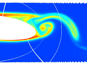
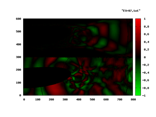
The wake of an obstacle in the flow may develop a Kármán vortex street. The Fig.1 shows the shedding of a vortex behind the trailing edge of a profile. The DMD-analysis was applied to 90 sequential Entropy fields (animated gif (1.9MB) )and yield an approximated eigenvalue-spectrum as depicted below. The analysis was applied to the numerical results, without referring to the governing equations. The profile is seen in white. The white arcs are the processor boundaries since the computation was performed on a parallel computer using different computational blocks.

Fig.2 DMD-spectrum

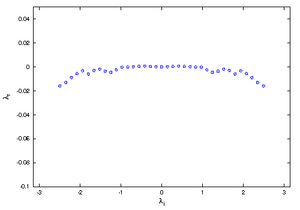
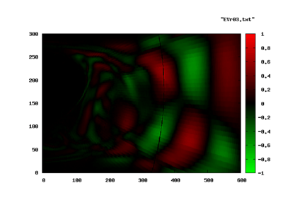
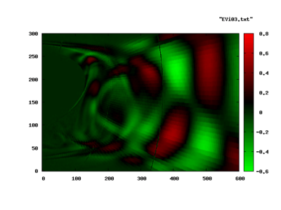
Roughly a third of the spectrum was highly damped (large, negative ${\displaystyle \lambda _{r}}$) and is not shown. The dominant shedding mode is shown in the following pictures. The image to the left is the real part, the image to the right, the imaginary part of the eigenvector.

Again, the entropy-eigenvector is shown in this picture. The acoustic contents of the same mode is seen in the bottom half of the next plot. The top half corresponds to the entropy mode as above.

Synthetic example of a traveling pattern

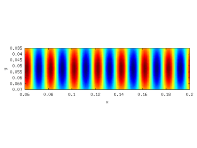
The DMD analysis assumes a pattern of the form ${\displaystyle q(x_{1},x_{2},x_{3},\ldots )=e^{cx_{1}}{\hat {q}}(x_{2},x_{3},\ldots )}$ where ${\displaystyle x_{1}}$ is any of the independent variables of the problem, but has to be selected in advance. Take for example the pattern

${\displaystyle q(x,y,t)=e^{-i\omega t}{\hat {q}}(x,t)e^{-(y/b)^{2}}\Re \left\{e^{i(kx-\omega t)}\right\}+{\text{random noise}}}$

With the time as the preselected exponential factor.

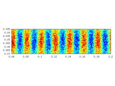
A sample is given in the following figure with ${\displaystyle \omega =2\pi /0.1}$, ${\displaystyle b=0.02}$ and ${\displaystyle k=2\pi /b}$. The left picture shows the pattern without, the right with noise added. The amplitude of the random noise is the same as that of the pattern.

A DMD analysis is performed with 21 synthetically generated fields using a time interval ${\displaystyle \Delta t=1/90{\text{ s}}}$, limiting the analysis to ${\displaystyle f=45{\text{ Hz}}}$.

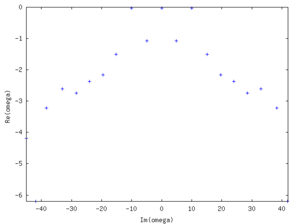
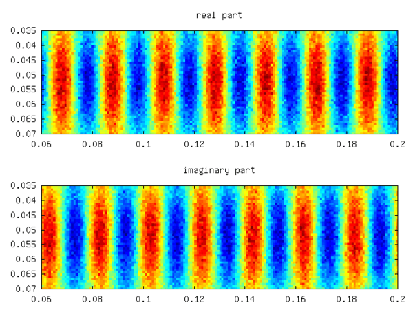
The spectrum is symmetric and shows three almost undamped modes (small negative real part), whereas the other modes are heavily damped. Their numerical values are ${\displaystyle \omega _{1}=-0.201,\omega _{2/3}=-0.223\pm i62.768}$ respectively. The real one corresponds to the mean of the field, whereas ${\displaystyle \omega _{2/3}}$ corresponds to the imposed pattern with ${\displaystyle f=10{\text{ Hz}}}$. Yielding a relative error of −1/1000. Increasing the noise to 10 times the signal value yields about the same error. The real and imaginary part of one of the latter two eigenmodes is depicted in the following figure.

See also

Several other decompositions of experimental data exist. If the governing equations are available, an eigenvalue decomposition might be feasible.

• Eigenvalue decomposition
• Empirical mode decomposition
• Global mode
• Normal mode
• Proper orthogonal decomposition
• Singular-value decomposition

References

1. P.J. Schmid. "Dynamic mode decomposition of numerical and experimental data." Journal of Fluid Mechanics 656.1 (2010): 5–28.
2. C.W. Rowley, I Mezic, S. Bagheri, P. Schlatter, and D.S. Henningson, "Spectral analysis of nonlinear flows." Journal of Fluid Mechanics 641 (2009): 85-113
3. K.K. Chen, J.H. Tu, and C.W. Rowley, "Variants of dynamic mode decomposition: boundary condition, Koopman, and Fourier analyses." Journal of Nonlinear Science 22 (2012): 887-915.
4. A. Wynn, D. S. Pearson, B. Ganapathisubramani and P. J. Goulart, "Optimal mode decomposition for unsteady flows." Journal of Fluid Mechanics 733 (2013): 473-503
5. Tu, Rowley, Luchtenburg, Brunton, and Kutz (December 2014). "On Dynamic Mode Decomposition: Theory and Applications". American Institute of Mathematical Sciences. arXiv:1312.0041. doi:10.3934/jcd.2014.1.391.CS1 maint: multiple names: authors list (link)
6. M.R. Jovanovic, P.J. Schmid, and J.W. Nichols, "Sparsity-promoting dynamic mode decomposition." Physics of Fluids 26 (2014)
7. J.N. Kutz, X. Fu, and S.L. Brunton, "Multi-resolution dynamic mode decomposition." arXiv preprint arXiv:1506.00564 (2015).
8. M.O. Williams , I.G. Kevrekidis, C.W. Rowley, "A Data–Driven Approximation of the Koopman Operator: Extending Dynamic Mode Decomposition." Journal of Nonlinear Science 25 (2015): 1307-1346.
9. J.L. Proctor, S.L. Brunton, and J.N. Kutz, "Dynamic mode decomposition with control." arXiv preprint arXiv:1409.6358 (2014).
10. M.S. Hemati, C.W. Rowley, E.A. Deem, and L.N. Cattafesta, "De-Biasing the Dynamic Mode Decomposition for Applied Koopman Spectral Analysis of Noisy Datasets." arXiv preprint arXiv:1502.03854 (2015).
11. Taylor-King, Jake P.; Riseth, Asbjørn N.; Macnair, Will; Claassen, Manfred (2020-01-10). "Dynamic distribution decomposition for single-cell snapshot time series identifies subpopulations and trajectories during iPSC reprogramming". PLOS Computational Biology. 16 (1): e1007491. doi:10.1371/journal.pcbi.1007491. ISSN 1553-7358. PMC 6953770. PMID 31923173.
12. Penland, Magorian, Cecile, Theresa (1993). "Prediction of Niño 3 Sea Surface Temperatures Using Linear Inverse Modeling". J. Climate. 6.

• Schmid, P. J. & Sesterhenn, J. L. 2008 Dynamic mode decomposition of numerical and experimental data. In Bull. Amer. Phys. Soc., 61st APS meeting, p. 208. San Antonio.
• Hasselmann, K., 1988. POPs and PIPs. The reduction of complex dynamical systems using principal oscillation and interaction patterns. J. Geophys. Res., 93(D9): 10975–10988.