Classical XY model

The classical XY model (sometimes also called classical rotor (rotator) model or O(2) model) is a lattice model of statistical mechanics. It is the special case of the n-vector model for n = 2.

Definition

Given a D-dimensional lattice Λ, per each lattice site j ∈ Λ there is a two-dimensional, unit-length vector s_j = (cos θ_j, sin θ_j)

The spin configuration, s = (s_j)_{j ∈ Λ} is an assignment of the angle −π < θ_j ≤ π for each j ∈ Λ.

Given a translation-invariant interaction J_ij = J(i − j) and a point dependent external field ${\displaystyle \mathbf {h} _{j}=(h_{j},0)}$, the configuration energy is

${\displaystyle H(\mathbf {s} )=-\sum _{i\neq j}J_{ij}\;\mathbf {s} _{i}\cdot \mathbf {s} _{j}-\sum _{j}\mathbf {h} _{j}\cdot \mathbf {s} _{j}=-\sum _{i\neq j}J_{ij}\;\cos(\theta _{i}-\theta _{j})-\sum _{j}h_{j}\cos \theta _{j}}$

The case in which J_ij = 0 except for ij nearest neighbor is called nearest neighbor case.

The configuration probability is given by the Boltzmann distribution with inverse temperature β ≥ 0:

${\displaystyle P(\mathbf {s} )={\frac {e^{-\beta H(\mathbf {s} )}}{Z}}\qquad Z=\int _{[-\pi ,\pi ]^{\Lambda }}\prod _{j\in \Lambda }d\theta _{j}\;e^{-\beta H(\mathbf {s} )}.}$

where Z is the normalization, or partition function.[1] The notation ${\displaystyle \langle A(\mathbf {s} )\rangle }$ indicates the expectation of the random variable A(s) in the infinite volume limit, after periodic boundary conditions have been imposed.

General properties

• The existence of the thermodynamic limit for the free energy and spin correlations were proved by Ginibre, extending to this case the Griffiths inequality.[2]
• Using the Griffiths inequality in the formulation of Ginibre, Aizenman and Simon[3] proved that the two point spin correlation of the ferromagnetics XY model in dimension D, coupling J > 0 and inverse temperature β is dominated by (i.e. has an upper bound given by) the two point correlation of the ferromagnetic Ising model in dimension D, coupling J > 0 and inverse temperature β/2

${\displaystyle \langle \mathbf {s} _{i}\cdot \mathbf {s} _{j}\rangle _{J,2\beta }\leq \langle \sigma _{i}\sigma _{j}\rangle _{J,\beta }}$

Hence the critical β of the XY model cannot be smaller than the double of the critical temperature of the Ising model

${\displaystyle \beta _{c}^{XY}\geq 2\beta _{c}^{\rm {Is}}}$

One dimension

As in any 'nearest-neighbor' n-vector model with free (non-periodic) boundary conditions, if the external field is zero, there exists a simple exact solution. In the free boundary conditions case, the Hamiltonian is

${\displaystyle H(\mathbf {s} )=-J[\cos(\theta _{1}-\theta _{2})+\cdots +\cos(\theta _{L-1}-\theta _{L})]}$

therefore the partition function factorizes under the change of coordinates

${\displaystyle \theta _{j}=\theta _{j}'+\theta _{j-1}\qquad j\geq 2}$

This gives

Exact specific heat per spin in the one-dimensional XY model

${\displaystyle {\begin{aligned}Z&=\int _{-\pi }^{\pi }d\theta _{1}\cdots d\theta _{L}\;e^{\beta J\cos(\theta _{1}-\theta _{2})}\cdots e^{\beta J\cos(\theta _{L-1}-\theta _{L})}\\&=2\pi \prod _{j=2}^{L}\int _{-\pi }^{\pi }d\theta '_{j}\;e^{\beta J\cos \theta '_{j}}=(2\pi )\left[\int _{-\pi }^{\pi }d\theta '_{j}\;e^{\beta J\cos \theta '_{j}}\right]^{L-1}=(2\pi )^{L}(I_{0}(\beta J))^{L-1}\end{aligned}}}$

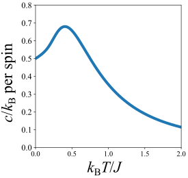
where ${\displaystyle I_{0}}$ is the modified Bessel function of the first kind. The partition function can be used to find several important thermodynamic quantities. For example, in the thermodynamic limit (${\displaystyle L\to \infty }$), the free energy per spin is

${\displaystyle f(\beta ,h=0)=-\lim _{L\to \infty }{\frac {1}{\beta L}}\ln Z=-{\frac {1}{\beta }}\ln[2\pi I_{0}(\beta J)]}$

Using the properties of the modified Bessel functions, the specific heat (per spin) can be expressed as[4]

${\displaystyle {\frac {c}{k_{B}}}=\lim _{L\to \infty }{\frac {1}{L(k_{B}T)^{2}}}{\frac {\partial ^{2}}{\partial \beta ^{2}}}(\ln Z)=K^{2}\left(1-{\frac {\mu }{K}}-\mu ^{2}\right)}$

where ${\displaystyle K=J/k_{B}T}$, and ${\displaystyle \mu }$ is the short-range correlation function,

${\displaystyle \mu (K)=\langle \cos(\theta -\theta ')\rangle ={\frac {I_{1}(K)}{I_{0}(K)}}}$

Even in the thermodynamic limit, there is no divergence in the specific heat. Indeed, like the one-dimensional Ising model, the one-dimensional XY model has no phase transitions at finite temperature.

The same computation for periodic boundary condition (and still h = 0) requires the transfer matrix formalism, though the result is the same.[5].

(Click "show" at right to see the details of the transfer matrix formalism.)

The partition function can be evaluated as

${\displaystyle Z={\text{tr}}\left\{\prod _{i=1}^{N}\oint d\theta _{i}e^{\beta J\cos(\theta _{i}-\theta _{i+1})}\right\}}$

which can be treated as the trace of a matrix, namely a product of matrices (scalars, in this case). The trace of a matrix is simply the sum of its eigenvalues, and in the thermodynamic limit ${\displaystyle L\to \infty }$ only the largest eigenvalue will survive, so the partition function can be written as a repeated product of this maximal eigenvalue. This requires solving the eigenvalue problem

${\displaystyle \oint d\theta '\exp\{\beta J\cos(\theta '-\theta )\}\psi (\theta ')=z_{i}\psi (\theta )}$

Note the expansion

${\displaystyle \exp\{\beta J\cos(\theta -\theta ')\}=\sum _{n=-\infty }^{\infty }I_{n}(\beta J)e^{in(\theta -\theta ')}=\sum _{n=-\infty }^{\infty }\omega _{n}\psi _{n}^{*}(\theta ')\psi _{n}(\theta )}$

which represents a diagonal matrix representation in the basis of its plane-wave eigenfunctions ${\displaystyle \psi =\exp(in\theta )}$. The eigenvalues of the matrix is simply are modified Bessel functions evaluated at ${\displaystyle \beta J}$, namely ${\displaystyle \omega _{n}=2\pi I_{n}(\beta J)}$. For any particular value of ${\displaystyle \beta J}$, these modified Bessel functions satisfy ${\displaystyle I_{0}>I_{1}>I_{2}>\cdots }$ and ${\displaystyle I_{-n}(\beta J)=I_{n}(\beta J)}$. Therefore in the thermodynamic limit the eigenvalue ${\displaystyle I_{0}}$ will dominate the trace, and so ${\displaystyle Z=[2\pi I_{0}(\beta J)]^{L}}$.

This transfer matrix approach is also required when using free boundary conditions, but with an applied field ${\displaystyle h\neq 0}$. If the applied field ${\displaystyle h}$ is small enough that it can be treated as a perturbation to the system in zero-field, then the magnetic susceptibility ${\displaystyle \chi \equiv \partial M/\partial h}$ can be estimated. This is done by using the eigenstates computed by the transfer matrix approach and computing the energy shift with second-order perturbation theory, then comparing with the free-energy expansion ${\displaystyle F=F_{0}-{\frac {1}{2}}\chi h^{2}}$. One finds [6]

${\displaystyle \chi (h\to 0)={\frac {C}{T}}{\frac {1+\mu }{1-\mu }}}$

where ${\displaystyle C}$ is the Curie constant (a value typically associated with the susceptibility in magnetic materials). This expression is also true for the one-dimensional Ising model, with the replacement ${\displaystyle \mu =\tanh K}$.

Two dimensions

Mean-square mganetization for a 25x25 lattice (Ota[7]: 30x30), suggesting an increase in magnetic moment that is not present in the thermodynamic limit

The two-dimensional XY model with nearest-neighbor interactions is an example of a two-dimensional system with continuous symmetry that does not have long-range order as required by the Mermin–Wagner theorem. Likewise, there is not a conventional phase transition present that would be associated with symmetry breaking. However, as will be discussed later, the system does show signs of a transition from a disordered high-temperature state to a quasi-ordered state below some critical temperature, called the Kosterlitz-Thouless transition. In the case of a discrete lattice of spins, two-dimensional XY model can be evaluated using the transfer matrix approach, reducing the model to an eigenvalue problem and utilizing the largest eigenvalue from the transfer matrix. Though the exact solution is intractable, it is possible to use certain approximations to get estimates for the critical temperature ${\displaystyle T_{c}}$ which occurs at low temperatures. For example, Mattis (1984) used an approximation to this model to estimate a critical temperature of the system as

${\displaystyle (2k_{B}T_{c}/J)\ln(2k_{B}T_{c}/J)=1}$

${\displaystyle k_{B}T_{c}/J\approx 0.8816}$

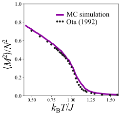
The 2D XY model has also been studied in great detail using Monte Carlo simulations, for example with the Metropolis algorithm. These can be used to compute thermodynamic quantities like the system energy, specific heat, magnetization, etc., over a range of temperatures and time-scales. In the Monte Carlo simulation, each spin is associated to a continuously-varying angle ${\displaystyle \theta _{i}}$ (often, it can be discretized into finitely-many angles, like in the related Potts model, for ease of computation. However, this is not a requirement.) At each time step the Metropolis algorithm chooses one spin at random and rotates its angle by some random increment ${\displaystyle \Delta \theta _{i}\in (-\Delta ,\Delta )}$. This change in angle causes a change in the energy ${\displaystyle \Delta E_{i}}$ of the system, which can be positive or negative. If negative, the algorithm accepts the change in angle; if negative, the configuration is accepted with probability ${\displaystyle e^{-\beta \Delta E_{i}}}$, the Boltzmann factor for the energy change. The Monte Carlo method has been used to verify, with various methods, the critical temperature of the system, and is estimated to be[8] ${\displaystyle k_{B}T_{c}/J=0.8935(1)}$. The Monte Carlo method can also compute average values that are used to compute thermodynamic quantities like magnetization, spin-spin correlation, correlation lengths, and specific heat. These are important ways to characterize the behavior of the system near the critical temperature. The magnetization and squared magnetization, for example, can be computed as

Specific heat of the two-dimensional XY using a Monte Carlo simulation, showing a feature at ${\displaystyle k_{B}T/J\approx 1.1}$, above the K-T transition

${\displaystyle {\frac {\langle M\rangle }{N}}={\frac {1}{N}}|\langle \mathbf {s} \rangle |={\frac {1}{N}}{\Bigg |}\left\langle \left(\sum _{i=1}^{N}\cos \theta _{i},\sum _{i=1}^{N}\sin \theta _{i}\right)\right\rangle {\Bigg |}}$

${\displaystyle {\frac {\langle M^{2}\rangle }{N^{2}}}={\frac {1}{N^{2}}}\left\langle s_{x}^{2}+s_{y}^{2}\right\rangle ={\frac {1}{N^{2}}}\left\langle \left(\sum _{i=1}^{N}\cos \theta _{i}\right)^{2}+\left(\sum _{i=1}^{N}\sin \theta _{i}\right)^{2}\right\rangle }$

where ${\displaystyle N=L\times L}$ are the number of spins. The mean magnetization characterizes the magnitude of the net magnetic moment of the system; in many magnetic systems this is zero above a critical temperature and becomes non-zero spontaneously at low temperatures. Similarly the mean-squared magnetization characterizes the average of the square of net components of the spins across the lattice. Either of these are commonly used to characterize the order parameter of a system. Rigorous analysis of the XY model shows the magnetization in the thermodynamic limit is zero, and that the square magnetization approximately follows[9] ${\displaystyle \langle M^{2}\rangle \approx N^{-T/4\pi }}$, which vanishes in the thermodynamic limit. Indeed, at high temperatures this quantity approaches zero since the components of the spins will tend to be randomized and thus sum to zero. However at low temperatures for a finite system, the mean-square magnetization increases, suggesting there are regions of the spin space that are aligned to contribute to a non-zero contribution. The magnetization shown (for a 25x25 lattice) is one example of this, that appears to suggest a phase transition, while no such transition exists in the thermodynamic limit.

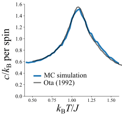
Furthermore, using statistical mechanics one can relate thermodynamic averages to quantities like specific heat by calculating

${\displaystyle c/k_{B}={\frac {\langle E^{2}\rangle -\langle E\rangle ^{2}}{N(k_{B}T)^{2}}}}$

The specific heat is shown at low temperatures near the critical temperature ${\displaystyle k_{B}T_{c}/J\approx 0.88}$. There is no feature in the specific heat consistent with a critical feature (like a divergence) at this predicted temperature. Indeed, estimating the critical temperature comes from other methods, like from the helicity modulus, or the temperature dependence of the divergence of susceptibility[10]. However, there is a feature in the specific heat in the form of a peak near ${\displaystyle 1.1k_{B}T/J}$. This peak position and peak height has been shown to depend on the system size[11]; however, the feature remains finite for all lattice sizes and appears to converge to a finite value (although the feature being a cusp has not been ruled out, this is unlikely).

The nature of the critical transitions and vortex formation can be elucidated by considering a continuous version of the XY model. Here, the discrete spins ${\displaystyle \theta _{n}}$ are replaced by a field ${\displaystyle \theta ({\textbf {x}})}$ representing the spin's angle at any point in space. In this case the angle of the spins ${\displaystyle \theta ({\textbf {x}})}$ must vary smoothly over changes in position. Expanding the original cosine as a Taylor series, the Hamiltonian can be expressed in the continuum approximation as

${\displaystyle E=\int {\frac {J}{2}}(\nabla \theta )^{2}\,d^{2}{\textbf {x}}}$

Color map of the (discrete) two-dimensional XY model in a 250x250 lattice at ${\displaystyle k_{B}T/J=0.4}$. Each spin is represented by a color that corresponds to an angle between ${\displaystyle (-\pi ,\pi ]}$

The continuous version of the XY model is often used to model systems that possess order parameters with the same kinds of symmetry, e.g. superfluid helium, hexatic liquid crystals. This is what makes them peculiar from other phase transitions which are always accompanied with a symmetry breaking. Topological defects in the XY model lead to a vortex-unbinding transition from the low-temperature phase to the high-temperature disordered phase. Indeed, the fact that at high temperature correlations decay exponentially fast, while at low temperatures decay with power law, even though in both regimes M(β) = 0, is called Kosterlitz–Thouless transition. Kosterlitz and Thouless provided a simple argument of why this would be the case: this considers the ground state consisting of all spins in the same orientation, with the addition then of a single vortex. The presence of these contributes an entropy of roughly ${\displaystyle \Delta S=k_{B}\ln(L^{2}/a^{2})}$, where ${\displaystyle a}$ is an effective length scale (for example, the lattice size for a discrete lattice) Meanwhile, the energy of the system increases due to the vortex, by an amount ${\displaystyle \Delta E=\pi J\ln(L/a)}$. Putting these together, the free energy of a system would change due to the spontaneous formation of a vortex by an amount

${\displaystyle \Delta F=\Delta E-T\Delta S=(\pi J-2k_{B}T)\ln(L/a)}$

In the thermodynamic limit, the system does not favor the formation of vortices at low temperatures, but does favor them at high temperatures, above the critical temperature ${\displaystyle T_{c}=\pi J/2k_{B}}$. This indicates that at low temperatures, any vortices that arise will want to annihilate with antivortices to lower the system energy. Indeed, this will be the case qualitatively if one watches 'snapshots' of the spin system at low temperatures, where vortices and antivortices gradually come together to annihilate. Thus, the low-temperature state will consist of bound vortex-antivortex pairs. Meanwhile at high temperatures, there will be a collection of unbound vortices and antivortices that are free to move about the plane.

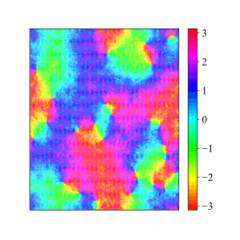
To visualize the Ising model, one can use an arrow pointing up or down, or represented as a point colored black/white to indicate its state. To visualize the XY spin system, the spins can be represented as an arrow pointing in some direction, or as being represented as a point with some color. Here it is necessary to represent the spin with a spectrum of colors due to each of the possible continuous variables. This can be done using, for example, a continuous and periodic red-green-blue spectrum. As shown on the figure, cyan corresponds to a zero angle (pointing to the right), whereas red corresponds to a 180 degree angle (pointing to the left). One can then study snapshots of the spin configurations at different temperatures to elucidate what happens above and below the critical temperature of the XY model. At high temperatures, the spins will not have a preferred orientation and there will be unpredictable variation of angles between neighboring spins, as there will be no preferred energetically favorable configuration. In this case, the color map will look highly pixellated. Meanwhile at low temperatures, one possible ground-state configuration has all spins pointed in the same orientation (same angle); these would correspond to regions (domains) of the color map where all spins have roughly the same color.

Various forms of vortices and antivortices, shown in a Monte Carlo simulation at ${\displaystyle k_{B}T/J=0.4}$

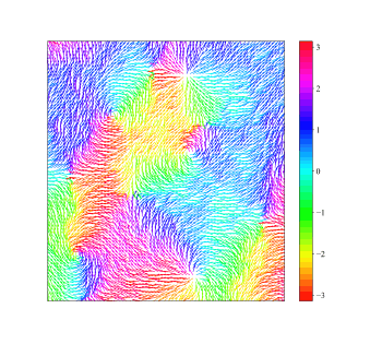
To identify vortices (or antivortices) present as a result of the Kosterlitz–Thouless transition, one can determine the signed change in angle by traversing a circle of lattice points counterclockwise. If the total change in angle is zero, this corresponds to no vortex being present; whereas a total change in angle of ${\displaystyle \pm 2\pi }$ corresponds to a vortex (or antivortex). These vortexes are topologically non-trivial objects that come in vortex-antivortex pairs, which can separate or pair-annihilate. In the colormap, these defects can be identified in regions where there is a large color gradient where all colors of the spectrum meet around a point. Qualitatively, these defects can look like inward- or outward-pointing sources of flow, or whirlpools of spins that collectively clockwise or counterclockwise, or hyperbolic-looking features with some spins pointing toward and some spins pointing away from the defect. As the configuration is studied at long time scales and at low temperatures, it is observed that many of these vortex-antivortex pairs get closer together and eventually pair-annihilate. It is only at high temperatures that these vortices and antivortices are liberated and unbind from one another.

In the continuous XY model, the high-temperature spontaneous magnetization vanishes:

${\displaystyle M(\beta ):=|\langle \mathbf {s} _{i}\rangle |=0}$

Besides, cluster expansion shows that the spin correlations cluster exponentially fast: for instance

${\displaystyle |\langle \mathbf {s} _{i}\cdot \mathbf {s} _{j}\rangle |\leq C(\beta )e^{-c(\beta )|i-j|}}$

At low temperatures, i.e. β ≫ 1, the spontaneous magnetization remains zero (see the Mermin–Wagner theorem),

${\displaystyle M(\beta ):=|\langle \mathbf {s} _{i}\rangle |=0}$

but the decay of the correlations is only power law: Fröhlich and Spencer[12] found the lower bound

${\displaystyle |\langle \mathbf {s} _{i}\cdot \mathbf {s} _{j}\rangle |\geq {\frac {C(\beta )}{1+|i-j|^{\eta (\beta )}}}}$

while McBryan and Spencer found the upper bound, for any ${\displaystyle \epsilon >0}$

${\displaystyle |\langle \mathbf {s} _{i}\cdot \mathbf {s} _{j}\rangle |\leq {\frac {C(\beta ,\epsilon )}{1+|i-j|^{\eta (\beta ,\epsilon )}}}}$

Three and higher dimensions

Independently of the range of the interaction, at low enough temperature the magnetization is positive.

• At high temperature, the spontaneous magnetization vanishes:

${\displaystyle M(\beta ):=|\langle \mathbf {s} _{i}\rangle |=0}$

Besides, cluster expansion shows that the spin correlations cluster exponentially fast: for instance

${\displaystyle |\langle \mathbf {s} _{i}\cdot \mathbf {s} _{j}\rangle |\leq C(\beta )e^{-c(\beta )|i-j|}}$

• At low temperature, infrared bound shows that the spontaneous magnetization is strictly positive:

${\displaystyle M(\beta ):=|\langle \mathbf {s} _{i}\rangle |>0}$

Besides, there exists a 1-parameter family of extremal states, ${\displaystyle \langle \;\cdot \;\rangle ^{\theta }}$, such that

${\displaystyle \langle \mathbf {s} _{i}\rangle ^{\theta }=M(\beta )(\cos \theta ,\sin \theta )}$

but, conjecturally, in each of these extremal states the truncated correlations decay algebraically.

In general, the XY model can be seen as a specialization of Stanley's n-vector model [13]

See also

• Classical Heisenberg model
• Goldstone boson
• Ising model
• Potts model
• n-vector model
• Kosterlitz–Thouless transition
• Topological defect
• Superfluid film

Notes

1. Chaikin, P.M.; Lubensky, T.C. (2000). Principles of Condensed Matter Physics. Cambridge University Press. ISBN 978-0521794503.
2. Ginibre, J. (1970). "General formulation of Griffiths' inequalities". Comm. Math. Phys. 16 (4): 310–328. Bibcode:1970CMaPh..16..310G. doi:10.1007/BF01646537.
3. Aizenman, M.; Simon, B. (1980). "A comparison of plane rotor and Ising models". Phys. Lett. A. 76 (3–4): 281–282. Bibcode:1980PhLA...76..281A. doi:10.1016/0375-9601(80)90493-4.
4. Badalian, D. (1996). "On the thermodynamics of classical spins with isotrop Heisenberg interaction in one-dimensional quasi-periodic structures". Physica B. 226: 385–390. doi:10.1016/0921-4526(96)00283-9.
5. Mattis, D.C. (1984). "Transfer matrix in plane-rotator model". Phys. Lett. 104 A (6–7): 357–360. Bibcode:1984PhLA..104..357M. doi:10.1016/0375-9601(84)90816-8.
6. Mattis, D. C. (1985). The Theory of Magnetism II. Springer Series in Solid-State Physics. ISBN 978-3-642-82405-0.
7. Ota, S.; Ota, S.B.; Fahnle, M (1992). "Microcanonical Monte Carlo simulations for the two-dimensional XY model". J. Phys.: Condens. Matter. 4: 5411. doi:10.1088/0953-8984/4/24/011.
8. Hsieh, Y.-D.; Kao, Y.-J.; Sandvik, A.W. (2013). "Finite-size scaling method for the Berezinskii-Kosterlitz-Thouless transition". J. Stat. Mech.: Theory Exp. 2013. arXiv:1302.2900. doi:10.1088/1742-5468/2013/09/P09001.
9. Tobochnik, J.; Chester, G.V. (1979). "Monte Carlo study of the planar spin model". Phys. Rev. B. 20 (9): 3761–3769. doi:10.1103/PhysRevB.20.3761.
10. Binder, K. (2013). Applications of the Monte Carlo Method in Statistical Physics. Springer Science & Business Media. ISBN 978-3-642-51703-7.
11. Van Himbergen, J.E.; Chakravarty, Sudip (1981). "Helicity modulus and specific heat of classical XY model in two dimensions". Phys. Rev. B. 23: 359. doi:10.1103/PhysRevB.23.359.
12. Fröhlich, J.; Spencer, T. (1981). "The Kosterlitz–Thouless transition in two-dimensional abelian spin systems and the Coulomb gas". Comm. Math. Phys. 81 (4): 527–602. Bibcode:1981CMaPh..81..527F. doi:10.1007/bf01208273.
13. Stanley, H.E. (1968). "Dependence of Critical Properties on Dimensionality of Spins". Phys. Rev. Lett. 20 (12): 589–592. Bibcode:1968PhRvL..20..589S. doi:10.1103/PhysRevLett.20.589.

References

• Evgeny Demidov, Vortices in the XY model (2004)

Further reading

• H. E. Stanley, Introduction to Phase Transitions and Critical Phenomena, (Oxford University Press, Oxford and New York 1971);
• H. Kleinert, Gauge Fields in Condensed Matter, Vol. I, " SUPERFLOW AND VORTEX LINES", pp. 1–742, Vol. II, "STRESSES AND DEFECTS", pp. 743–1456, World Scientific (Singapore, 1989); Paperback ISBN 9971-5-0210-0 (also available online: Vol. I and Vol. II)

External links

• real-time XY model WebGL simulation
• Interactive Monte Carlo simulation of the Ising, XY and Heisenberg models with 3D graphics (requires WebGL compatible browser)