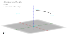
Centripetal Catmull–Rom spline

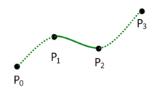
In computer graphics, centripetal Catmull–Rom spline is a variant form of Catmull-Rom spline, originally formulated by Edwin Catmull and Raphael Rom,[1] which can be evaluated using a recursive algorithm proposed by Barry and Goldman.[2] It is a type of interpolating spline (a curve that goes through its control points) defined by four control points ${\displaystyle \mathbf {P} _{0},\mathbf {P} _{1},\mathbf {P} _{2},\mathbf {P} _{3}}$, with the curve drawn only from ${\displaystyle \mathbf {P} _{1}}$ to ${\displaystyle \mathbf {P} _{2}}$.

Catmull–Rom spline interpolation with four points

Definition

Barry and Goldman's pyramidal formulation

Knot parameterization for the Catmull–Rom algorithm

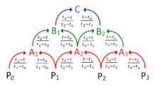
Let ${\displaystyle \mathbf {P} _{i}=[x_{i}\quad y_{i}]^{T}}$ denote a point. For a curve segment ${\displaystyle \mathbf {C} }$ defined by points ${\displaystyle \mathbf {P} _{0},\mathbf {P} _{1},\mathbf {P} _{2},\mathbf {P} _{3}}$ and knot sequence ${\displaystyle t_{0},t_{1},t_{2},t_{3}}$, the centripetal Catmull–Rom spline can be produced by:

${\displaystyle \mathbf {C} ={\frac {t_{2}-t}{t_{2}-t_{1}}}\mathbf {B} _{1}+{\frac {t-t_{1}}{t_{2}-t_{1}}}\mathbf {B} _{2}}$

where

${\displaystyle \mathbf {B} _{1}={\frac {t_{2}-t}{t_{2}-t_{0}}}\mathbf {A} _{1}+{\frac {t-t_{0}}{t_{2}-t_{0}}}\mathbf {A} _{2}}$

${\displaystyle \mathbf {B} _{2}={\frac {t_{3}-t}{t_{3}-t_{1}}}\mathbf {A} _{2}+{\frac {t-t_{1}}{t_{3}-t_{1}}}\mathbf {A} _{3}}$

${\displaystyle \mathbf {A} _{1}={\frac {t_{1}-t}{t_{1}-t_{0}}}\mathbf {P} _{0}+{\frac {t-t_{0}}{t_{1}-t_{0}}}\mathbf {P} _{1}}$

${\displaystyle \mathbf {A} _{2}={\frac {t_{2}-t}{t_{2}-t_{1}}}\mathbf {P} _{1}+{\frac {t-t_{1}}{t_{2}-t_{1}}}\mathbf {P} _{2}}$

${\displaystyle \mathbf {A} _{3}={\frac {t_{3}-t}{t_{3}-t_{2}}}\mathbf {P} _{2}+{\frac {t-t_{2}}{t_{3}-t_{2}}}\mathbf {P} _{3}}$

and

${\displaystyle t_{i+1}=\left[{\sqrt {(x_{i+1}-x_{i})^{2}+(y_{i+1}-y_{i})^{2}}}\right]^{\alpha }+t_{i}}$

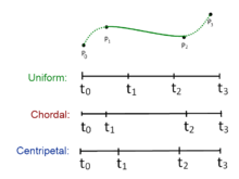
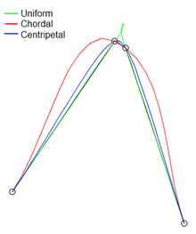
in which ${\displaystyle \alpha }$ ranges from 0 to 1 for knot parameterization, and ${\displaystyle i=0,1,2,3}$ with ${\displaystyle t_{0}=0}$. For centripetal Catmull–Rom spline, the value of ${\displaystyle \alpha }$ is ${\displaystyle 0.5}$. When ${\displaystyle \alpha =0}$, the resulting curve is the standard uniform Catmull–Rom spline; when ${\displaystyle \alpha =1}$, the product is a chordal Catmull–Rom spline.

Gif animation for uniform, centripetal and chordal parameterization of Catmull–Rom spline depending on the α value

Plugging ${\displaystyle t=t_{1}}$ into the spline equations ${\displaystyle \mathbf {A} _{1},\mathbf {A} _{2},\mathbf {A} _{3},\mathbf {B} _{1},\mathbf {B} _{2},}$ and ${\displaystyle \mathbf {C} }$ shows that the value of the spline curve at ${\displaystyle t_{1}}$ is ${\displaystyle \mathbf {C} =\mathbf {P} _{1}}$. Similarly, substituting ${\displaystyle t=t_{2}}$ into the spline equations shows that ${\displaystyle \mathbf {C} =\mathbf {P} _{2}}$ at ${\displaystyle t_{2}}$. This is true independent of the value of ${\displaystyle \alpha }$ since the equation for ${\displaystyle t_{i+1}}$ is not needed to calculate the value of ${\displaystyle \mathbf {C} }$ at points ${\displaystyle t_{1}}$ and ${\displaystyle t_{2}}$.

3D centripetal Catmull-Rom spline segment.

The extension to 3D points is simply achieved by considering ${\displaystyle \mathbf {P} _{i}=[x_{i}\quad y_{i}\quad z_{i}]^{T}}$a generic 3D point ${\displaystyle \mathbf {P} _{i}}$ and

${\displaystyle t_{i+1}=\left[{\sqrt {(x_{i+1}-x_{i})^{2}+(y_{i+1}-y_{i})^{2}+(z_{i+1}-z_{i})^{2}}}\right]^{\alpha }+t_{i}}$

Advantages

Centripetal Catmull–Rom spline has several desirable mathematical properties compared to the original and the other types of Catmull-Rom formulation.[3] First, it will not form loop or self-intersection within a curve segment. Second, cusp will never occur within a curve segment. Third, it follows the control points more tightly.

In this figure, there is a self-intersection/loop on the uniform Catmull-Rom spline (green), whereas for chordal Catmull-Rom spline (red), the curve does not follow tightly through the control points.

Other uses

In computer vision, centripetal Catmull-Rom spline has been used to formulate an active model for segmentation. The method is termed active spline model.[4] The model is devised on the basis of active shape model, but uses centripetal Catmull-Rom spline to join two successive points (active shape model uses simple straight line), so that the total number of points necessary to depict a shape is less. The use of centripetal Catmull-Rom spline makes the training of a shape model much simpler, and it enables a better way to edit a contour after segmentation.

Code example in Python

The following is an implementation of the Catmull–Rom spline in Python.

import numpy
import pylab as plt

def CatmullRomSpline(P0, P1, P2, P3, nPoints=100):
    """
    P0, P1, P2, and P3 should be (x,y) point pairs that define the Catmull-Rom spline.
    nPoints is the number of points to include in this curve segment.
    """
    # Convert the points to numpy so that we can do array multiplication
    P0, P1, P2, P3 = map(numpy.array, [P0, P1, P2, P3])

    # Parametric constant: 0.5 for the centripetal spline, 0.0 for the uniform spline, 1.0 for the chordal spline.
    alpha = 0.5
    # Premultiplied power constant for the following tj() function.
    alpha = alpha/2
    def tj(ti, Pi, Pj):
        xi, yi = Pi
        xj, yj = Pj
        return ((xj-xi)**2 + (yj-yi)**2)**alpha + ti

    # Calculate t0 to t4
    t0 = 0
    t1 = tj(t0, P0, P1)
    t2 = tj(t1, P1, P2)
    t3 = tj(t2, P2, P3)

    # Only calculate points between P1 and P2
    t = numpy.linspace(t1, t2, nPoints)

    # Reshape so that we can multiply by the points P0 to P3
    # and get a point for each value of t.
    t = t.reshape(len(t), 1)
    print(t)
    A1 = (t1-t)/(t1-t0)*P0 + (t-t0)/(t1-t0)*P1
    A2 = (t2-t)/(t2-t1)*P1 + (t-t1)/(t2-t1)*P2
    A3 = (t3-t)/(t3-t2)*P2 + (t-t2)/(t3-t2)*P3
    print(A1)
    print(A2)
    print(A3)
    B1 = (t2-t)/(t2-t0)*A1 + (t-t0)/(t2-t0)*A2
    B2 = (t3-t)/(t3-t1)*A2 + (t-t1)/(t3-t1)*A3

    C = (t2-t)/(t2-t1)*B1 + (t-t1)/(t2-t1)*B2
    return C

def CatmullRomChain(P):
    """
    Calculate Catmull–Rom for a chain of points and return the combined curve.
    """
    sz = len(P)

    # The curve C will contain an array of (x, y) points.
    C = []
    for i in range(sz-3):
        c = CatmullRomSpline(P[i], P[i+1], P[i+2], P[i+3])
        C.extend(c)

    return C

# Define a set of points for curve to go through
Points = [[0, 1.5], [2, 2], [3, 1], [4, 0.5], [5, 1], [6, 2], [7, 3]]

# Calculate the Catmull-Rom splines through the points
c = CatmullRomChain(Points)

# Convert the Catmull-Rom curve points into x and y arrays and plot
x, y = zip(*c)
plt.plot(x, y)

# Plot the control points
px, py = zip(*Points)
plt.plot(px, py, 'or')

plt.show()

Code example in Unity C#

using UnityEngine;
using System.Collections;
using System.Collections.Generic;

public class Catmul : MonoBehaviour {

	// Use the transforms of GameObjects in 3d space as your points or define array with desired points
	public Transform[] points;
	
	// Store points on the Catmull curve so we can visualize them
	List<Vector2> newPoints = new List<Vector2>();
	
	// How many points you want on the curve
	uint numberOfPoints = 10;
	
	// Parametric constant: 0.0 for the uniform spline, 0.5 for the centripetal spline, 1.0 for the chordal spline
	public float alpha = 0.5f;
	
	/////////////////////////////
	
	void Update()
	{
	    CatmulRom();
	}
	
	void CatmulRom()
	{
		newPoints.Clear();

		Vector2 p0 = points[0].position; // Vector3 has an implicit conversion to Vector2
		Vector2 p1 = points[1].position;
		Vector2 p2 = points[2].position;
		Vector2 p3 = points[3].position;

		float t0 = 0.0f;
		float t1 = GetT(t0, p0, p1);
		float t2 = GetT(t1, p1, p2);
		float t3 = GetT(t2, p2, p3);

		for (float t=t1; t<t2; t+=((t2-t1)/(float)numberOfPoints))
		{
		    Vector2 A1 = (t1-t)/(t1-t0)*p0 + (t-t0)/(t1-t0)*p1;
		    Vector2 A2 = (t2-t)/(t2-t1)*p1 + (t-t1)/(t2-t1)*p2;
		    Vector2 A3 = (t3-t)/(t3-t2)*p2 + (t-t2)/(t3-t2)*p3;
		    
		    Vector2 B1 = (t2-t)/(t2-t0)*A1 + (t-t0)/(t2-t0)*A2;
		    Vector2 B2 = (t3-t)/(t3-t1)*A2 + (t-t1)/(t3-t1)*A3;
		    
		    Vector2 C = (t2-t)/(t2-t1)*B1 + (t-t1)/(t2-t1)*B2;
		    
		    newPoints.Add(C);
		}
	}

	float GetT(float t, Vector2 p0, Vector2 p1)
	{
	    float a = Mathf.Pow((p1.x-p0.x), 2.0f) + Mathf.Pow((p1.y-p0.y), 2.0f);
	    float b = Mathf.Pow(a, alpha * 0.5f);
	   
	    return (b + t);
	}
	
	// Visualize the points
	void OnDrawGizmos()
	{
	    Gizmos.color = Color.red;
	    foreach (Vector2 temp in newPoints)
	    {
	        Vector3 pos = new Vector3(temp.x, temp.y, 0);
	        Gizmos.DrawSphere(pos, 0.3f);
	    }
	}
}

For an implementation in 3D space, after converting Vector2 to Vector3 points, the first line of function GetT should be changed to this: Mathf.Pow((p1.x-p0.x), 2.0f) + Mathf.Pow((p1.y-p0.y), 2.0f) + Mathf.Pow((p1.z-p0.z), 2.0f);

See also

• Cubic Hermite splines

References

1. Catmull, Edwin; Rom, Raphael (1974). "A class of local interpolating splines". In Barnhill, Robert E.; Riesenfeld, Richard F. (eds.). Computer Aided Geometric Design. pp. 317–326. doi:10.1016/B978-0-12-079050-0.50020-5. ISBN 978-0-12-079050-0.
2. Barry, Phillip J.; Goldman, Ronald N. (August 1988). A recursive evaluation algorithm for a class of Catmull–Rom splines (PDF). Proceedings of the 15st Annual Conference on Computer Graphics and Interactive Techniques, SIGGRAPH 1988. 22. Association for Computing Machinery. pp. 199–204. doi:10.1145/378456.378511.
3. Yuksel, Cem; Schaefer, Scott; Keyser, John (July 2011). "Parameterization and applications of Catmull-Rom curves". Computer-Aided Design. 43 (7): 747–755. CiteSeerX 10.1.1.359.9148. doi:10.1016/j.cad.2010.08.008.
4. Jen Hong, Tan; Acharya, U. Rajendra (2014). "Active spline model: A shape based model-interactive segmentation" (PDF). Digital Signal Processing. 35: 64–74. arXiv:1402.6387. doi:10.1016/j.dsp.2014.09.002.

External links

• Catmull-Rom curve with no cusps and no self-intersections – implementation in Java
• Catmull-Rom curve with no cusps and no self-intersections – simplified implementation in C++
• Catmull-Rom splines – interactive generation via Python, in a Jupyter notebook