Arakawa grids

The Arakawa grid system depicts different ways to represent and compute orthogonal physical quantities (especially velocity- and mass-related quantities) on rectangular grids used for Earth system models for meteorology and oceanography. For example, the Weather Research and Forecasting Model uses the Arakawa Staggered C-Grid in its atmospheric calculations when using the ARW core. The five Arakawa grids (A-E) were first introduced in Arakawa and Lamb 1977.[1]

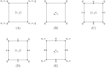
For an image of the five grids, see the following picture, or Fig. 1 in Purser and Leslie 1988.[2]

The five different grids by Arakawa

Arakawa A-grid

The "unstaggered" Arakawa A-grid evaluates all quantities at the same point on each grid cell, e.g., at the grid center or at the grid corners. The Arakawa A-grid is the only unstaggered grid type.

Arakawa B-grid

The "staggered" Arakawa B-grid separates the evaluation of the two sets of quantities. e.g., one might evaluate velocities at the grid center and masses at grid corners.

Arakawa C-grid

The "staggered" Arakawa C-grid further separates evaluation of vector quantities compared to the Arakawa B-grid. e.g., instead of evaluating both east-west (u) and north-south (v) velocity components at the grid center, one might evaluate the u components at the centers of the left and right grid faces, and the v components at the centers of the upper and lower grid faces.

Arakawa D-grid

An Arakawa D-grid is a 90° rotation of an Arakawa C-grid. E.g., instead of evaluating the v velocity components at the centers of the upper/lower grid faces and the u velocity components at the centers of the right/left grid faces, one would evaluate the v velocity components at the centers of the right/left grid faces and the u velocity components at the centers of the upper/lower grid faces.

Arakawa E-grid

The Arakawa E-grid is "staggered," but also rotated 45° relative to the other grid orientations. This allows all variables to be defined along a single face of the rectangular domain.

References

1. Arakawa, A.; Lamb, V.R. (1977). "Computational design of the basic dynamical processes of the UCLA general circulation model". Methods in Computational Physics: Advances in Research and Applications. 17: 173–265. doi:10.1016/B978-0-12-460817-7.50009-4. ISBN 9780124608177.
2. Purser, R. J.; Leslie, L. M. (October 1988). <2069:ASISLF>2.0.CO;2 "A Semi-Implicit, Semi-Lagrangian Finite-Difference Scheme Using Hligh-Order Spatial Differencing on a Nonstaggered Grid". Monthly Weather Review. 116 (10): 2069–2080. doi:10.1175/1520-0493(1988)116<2069:ASISLF>2.0.CO;2. ISSN 0027-0644.

Further reading

• Haltiner, G. J., and R. T. Williams, 1980. Numerical Prediction and Dynamic Meteorology. John Wiley and Sons, New York.