0
I have tried this, but I am unsuccessful. I have the data dump in an excel sheet (Excel 2010). The first column has month. The second has the dates. The third column has numerical data. I have applied filters on each column to get the data on the Pivot Table. There are entries for each date. There are sometimes multiple entries for a single date. Now, when I run the Pivot, I get the proper sum, but when I select average, the average is accurate only for the single entries associated with a date. I need to calculate average of multiple data entries for a single date. Here is an example:
November 11/1/13 30
November 11/2/13 25
November 11/3/13 20
November 11/3/13 25
Now, when I run the Pivot table and select to average the data, it calculates the average as (30+25+20+25)/4 = 20 (since there are 4 entries, so the sum gets divided by 4)
This is not desirable.
I require the calculation to be made as taking the 3rd and 4th entry as one for the date 11/3/13. So, the required output is (30+25+(20+25))/3 = 33.33.
I hope the example gives an clear idea of the requirement. I need a solution for this. How do we modify the Pivot so that the average is calculated not based on just the number of entries, but the average is calculated for the number of days.
Your suggestions are welcome.

Manan Badani
Posted 2014-01-10T07:26:21.613
Reputation: 1

Your question is not clear.
I have applied filters on each column to get the data on the Pivot Table-- What does that mean? In the pivot table, what are you using for the value field settings? Average or Sum? How come the pivot table still shows 4 values? If you have the date in the rows, then it will show only three values. If you average the value field, you'll see these three values: 30, 25, 22.5. And the grand total average of these is 25 – teylyn – 2014-01-10T09:52:15.247Hi, I have applied filters on the data dump sheet just to sort and have a column heading. Also, they appear as the PivotTable Field List. Can I have your e-mail ID, so that I can show you some screenshots. – Manan Badani – 2014-01-10T10:37:36.670
Please post a link to a workbook with some sample data. Replace confidential data with dummy text. Use a free file sharing service. And please mock up what you would like to see and describe the logic to arrive at that result. – teylyn – 2014-01-11T02:35:05.323
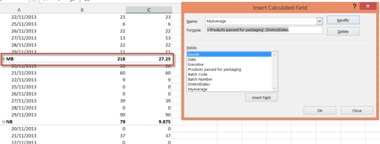
https://www.dropbox.com/sh/o77n3srmopg6ctf/NTvYTggUrW I have my file here. As you can see, in the Pivot, I have selected MB's data. I need the average as 27.25, and not 19.81. The denominator for average must be the number of days, and not the number of entries. MB's sum is 218. I need the answer as 218/8= 27.25, and not as 218/11= 19.81. Kindly provide a solution. Thank You. – Manan Badani – 2014-01-17T11:28:41.830