3
2
I'm having trouble with conditional formatting- so would really appreciate some guidance!
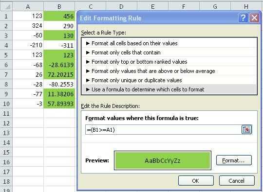
I want to format the numbers in column B, relative to the values in column A.
So if B is equal to or greater than A, format it green. If A is greater than B format it red.
(ahh i can't post an image!) Imagine for example:
Col A    Col B

  123     456

  324     290

   -50     130

 -210    -311

   123    123
Using the 'Greater Than' function i can achieve this on a row by row basis, but i can't figure out how to do this for a range of rows. So as in the example B1:B10 and A1:A10.
Similarly i can't combine the 'equal or greater than' with the 'less than' functions. But i guess that is simply a case of having two distinct rules that achieve the desired result.

Ned
Posted 2012-08-14T15:08:13.977
Reputation: 31

Do the comparison ranges change/grow or is it always 10 rows? – dav – 2012-08-14T16:13:05.227