How to get different color for different branches in a plot in MatLab, Mathematica and Desmos

Question

I am trying to obtain slab-waveguide dispersion plot like this (dashed line): I tried following code in Matlab:

function main
fimplicit (@(x,y)f(x,y),[0 10])
end
function fun = f(x,y)
nc=1.45;    %cladding
nf=1.5;
ns=1.4;    %substrate
h=5;  %width of waveguide
beta=sqrt(x^2*nf^2-y.^2);
gammas=sqrt(beta.^2-x^2*ns^2);
gammac=sqrt(beta.^2-x^2*nc^2);
z=sin(h*y);
%TE mode
fun=z-cos(h*y)*(gammac+gammas)./(y-gammas.*gammac./y);
end

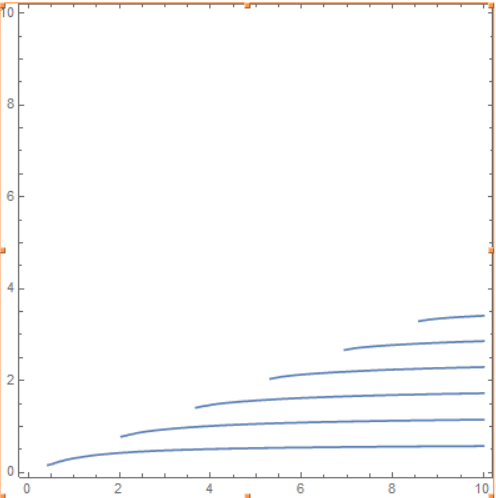
What I got:

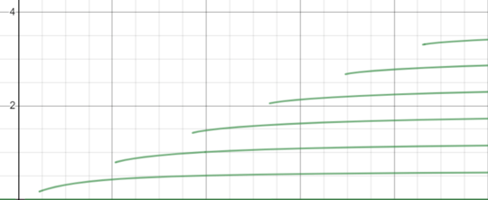
Using Desmos:

Using Mathematica:

nc = 1.45;
nf = 1.5;
ns = 1.4;
h = 5;
ContourPlot[
 Sin[h y]*(y^2 - (Sqrt[x^2*(nf^2 - nc^2) - y^2]*
       Sqrt[x^2*(nf^2 - ns^2) - y^2])) == 
  Cos[h y]*(Sqrt[x^2*(nf^2 - nc^2) - y^2] + 
     Sqrt[x^2*(nf^2 - ns^2) - y^2])*y, {x, 0, 10}, {y, 0.1, 10}]

All the plots are in excellent agreement with form expected. However the original plot has a different color for each branch, how can I implement this in MatLab, Desmos or Mathematica ?

Answer 1

Mathematica

Update

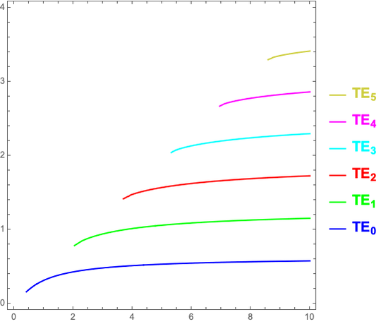
Add legend, use darker yellow color.

colors = {Blue, Green, Red, Cyan, Magenta, RGBColor["#cdcd41"]};

labels = MapThread[
   ToString[Subscript[Style["TE", Bold, 16, #2], 
      Style[ToString@#1, Bold, 12, #2]], StandardForm] &, {Range[0, 5], colors}];

legend = LineLegend[colors, labels, LegendLayout -> "ReversedColumn", LegendMarkerSize -> 20];

plot = ContourPlot[
   Sin[h y]*(y^2 - (Sqrt[x^2*(nf^2 - nc^2) - y^2]*
         Sqrt[x^2*(nf^2 - ns^2) - y^2])) == 
    Cos[h y]*(Sqrt[x^2*(nf^2 - nc^2) - y^2] + 
       Sqrt[x^2*(nf^2 - ns^2) - y^2])*y, {x, 0, 10}, {y, 0, 4}, PlotLegends -> legend];

coloredLines = Riffle[colors, Cases[plot, _Line, Infinity]];

plot /. {a___, Repeated[_Line, {6}], c___} :> {a, Sequence @@ coloredLines, c}

Original answer

I could not find a way to use ContourPlot options to color the lines of an implicit function plot. Here is a way (hack) to do it by post processing the plot expression.

plot = ContourPlot[
 Sin[h y]*(y^2 - (Sqrt[x^2*(nf^2 - nc^2) - y^2]*
       Sqrt[x^2*(nf^2 - ns^2) - y^2])) == 
  Cos[h y]*(Sqrt[x^2*(nf^2 - nc^2) - y^2] + 
     Sqrt[x^2*(nf^2 - ns^2) - y^2])*y, {x, 0, 10}, {y, 0, 4}];

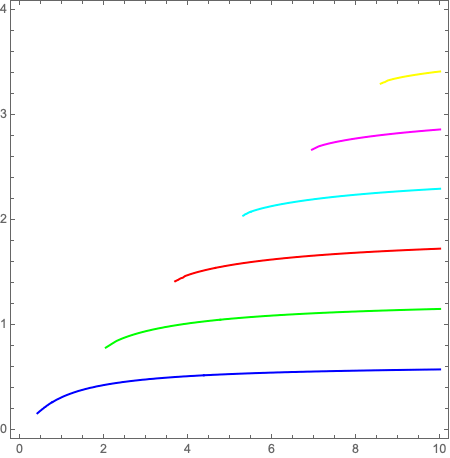
coloredLines = Riffle[{Blue, Green, Red, Cyan, Magenta, Yellow}, Cases[plot, _Line, Infinity]];

plot /. {a___, Repeated[_Line, {6}], c___} :> {a, Sequence @@ coloredLines, c}