Calculate additional values based on results of Pivot Table

Question

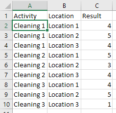
I am trying to make a summary of some cleaning results in Excel with the aid of a Pivot Table, but I am experiencing some troubles wrapping it all up. I have the following data:

Cleaning 1    Location 1    Result 1
Cleaning 1    Location 2    Result 2
Cleaning 1    Location 3    Result 3
Cleaning 2    Location 1    Result 4
Cleaning 2    Location 2    Result 5
Cleaning 2    Location 3    Result 6
Cleaning 3    Location 1    Result 7
Cleaning 3    Location 2    Result 8
Cleaning 3    Location 3    Result 9

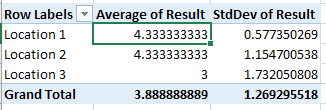
Currently, I have a Pivot Table containing the average and standard deviation of each location, as well as the average and standard deviation of all the results combined. I would also like to have average + 3 * standard deviationDaar for each location, as well as for all the results combined.

The info I find handles calculating additional paramaters based on the ORIGINAL columns of the data, but not combining RESULTING data in the Pivot Table. Any help?

What I have tried so far:

GETPIVOTDATA is a nice formula, but it does not work ideally for me since I will be using the filter options of the pivot table. Also, it does not seems to work for the total.

Answer 1

Unless you are going to do some VBA work, I think you are going to be stuck with GETPIVOTDATA. Below, I will show it does work, and how to make it work when you are messing with the filtering.

People are tempted to try to use Field Calculations. These work on a "row by row" basis, and you do not have access to the correct value for N or for STDEV. Again, I will demonstrate below.

Starting with this data, I put together from your question ...

... this Pivot Table was built ...

This Does Not Work

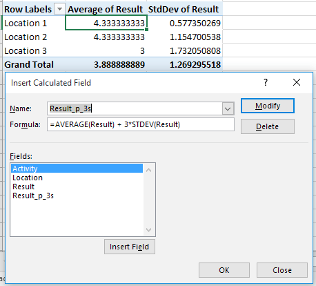
An attempt was made to create a Field Calculation ...

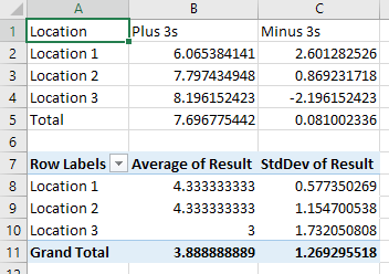
... with the following (erroneous) results ...

This Does Work

To implement spreadsheet calculations that will not be affected by changing the filtering on the Pivot Table, insert rows above the Pivot Table until you have enough room for the calculations you require.

For your example, the following was built ...

... A typical equation for Cells B2 through B4 is ...

=IF(ISERROR(GETPIVOTDATA("Average of Result",$A$7,$A$1,$A2)),"",GETPIVOTDATA("Average of Result",$A$7,$A$1,$A2)+3*GETPIVOTDATA("StdDev of Result",$A$7,$A$1,$A2))

... This equation checks if the Pivot Table contains information for "Location 1". If it does not, then nothing is displayed. If it does, then it adds 3 times the standard deviation for Location 1 to the average for Location 1.

Cells C2 through C4 are the same, except for subtraction. Cell B5 contains ...

=IF(ISERROR(GETPIVOTDATA("Average of Result",$A$7)),"",GETPIVOTDATA("Average of Result",$A$7)+3*GETPIVOTDATA("StdDev of Result",$A$7))

This equation checks if the Grand Total results are present. If they are not, nothing is displayed. If they are, then the grand total average + 3 times the grand total standard deviation is calculated.

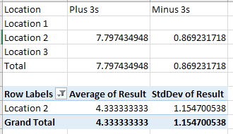
When the filtering is changed ...

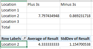
... when the Grand Totals are removed from the Pivot Table ...