1
I've got a conditional formatting question I'm really hoping someone can help with. I've got a workbook with 3 sheets - "Total Data", "Pivot Table" and "Expired Data". Pivot Table is extrapolated from Total Data. I want to analyze the data in Expired Data compared to the averages in Pivot Table.
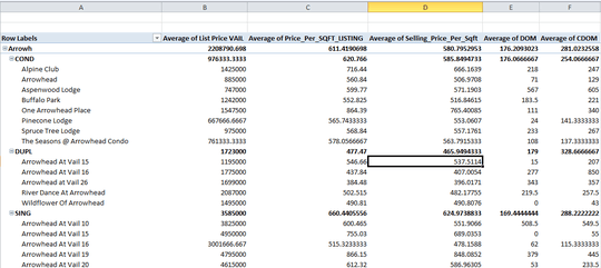
Pivot Table looks like this:
Expired Data looks like this:
In the PT column A contains labels - "Area", "Type", and "Subdivision" - and columns B-F are the values ("Avg. List Price", "Avg. List Price per SqFt", "Avg. Sale Price", "Avg. DOM" & "Avg. CDOM" respectively). I'm trying to use conditional formatting to ascertain whether the values in "Expired Data" (columns D-H in "Expired Data") are greater than or less than the averages in the PT, but first need to match the labels in column A (in order to compare like properties), recognizing the data in Expired Data may not be sorted.
If columns A-C of Expired Data match the labels in column A of the PT, I want the conditional formatting to turn RED those values that are greater than the corresponding averages on the PT, and ORANGE those values that are less than the corresponding averages on the PT. Layman formula = If A2, B2 & C2 are all contained in the same row in PT, then determine whether each value in Expired Data (List Price, List Price per SQFT, Sale Price, DOM and CDOM) is greater or less than the corresponding values in PT.
I've tried using vlookup in conditional formatting by going to Expired Data -> Conditional Formatting -> Highlight Cells -> Greater Than and using the following formula: =vlookup(c2,'Pivot Table'!$A:$A,2,0) to highlight list price on Expired Data that is greater than the average List Price for that complex on Pivot Table. Obviously I'm doing something wrong. Any help would be immensely appreciated!


THANK YOU - you're awesome! Almost there, but I need to match C2 & B2 on Expired Data (not just C2), as there are, for example, both Duplexes (DUPL) and Single Family Homes (SING) in the "Beaver Creek 2" Subdivision, so matching only "Beaver Creek 2" (Column C in Expired Data) returns the first match, which happens to be DUPL, but the property type on Expired Data is SING. I'm trying to use INDEX and MATCH, but can't figure out the greater than or less than part. I've edited my original post and have added pics. Again, THANK YOU VERY MUCH!!! – Andy Owen – 2016-01-14T16:24:36.663
sorry - it won't let me add new pictures, so I have not edited my original post. However, in the original post you'll see in the Pivot Table there are both DUPL and SING in Arrowh/Arrowhead at Vail 15, so I need to match both the property type (column B in Expired Data) and Subdivision (column C in Expired Data) to column A in Pivot Table. – Andy Owen – 2016-01-14T16:32:34.243
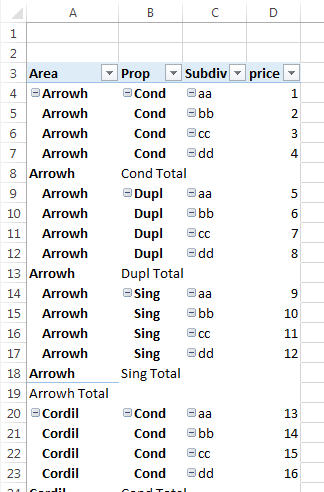
And next you want to add a third criterion, i.e. the Area. With the current pivot table layout this is not going to work. You need to use a tabular pivot table layout, so that the three criteria are in separate columns. I'll post a suggestion soon. – teylyn – 2016-01-14T21:27:32.820
I added a suggestion to my answer. – teylyn – 2016-01-14T21:51:46.297
YOU'RE AMAZING! I've been working on this for months - have posted the question on 4 different sites. You're the only one who could figure it out. Thank you SOOOO much! If you're ever in Colorado hit me up and I'll buy you a beer. – Andy Owen – 2016-01-14T22:55:46.807