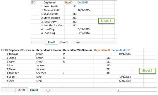
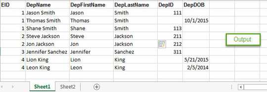
Solution as requested
A simple way to do this in the manner your requested is with helper columns. Lets say sheet 1 looks like your output example, with columns A:F shown, and sheet 2 is also showing A:F. Say we use column G for the helper column on each sheet.
The helper column concatenates the three comparison values. So on each sheet, G2 would contain:
=A2&E2&F2
Copy the formula down the column on each sheet. Then compare these values to find the record you need.
VLOOKUP requires that the lookup column be the leftmost in the array. You can accomplish the same style of lookup using INDEX plus MATCH, which doesn't have this limitation. Sheet 1, C2 would contain:
=INDEX(sheet2!B:C,MATCH(G2,sheet2!G:G,0),1)
and in D2:
=INDEX(sheet2!B:C,MATCH(G2,sheet2!G:G,0),2)
Copy these down the column. MATCH finds the key that matches the row on sheet 2 and returns the corresponding names.

You can hide the helper columns if you don't want to see them. If you're curious why the keys associated with a DepDOB don't look like a date it is because it uses the internal representation Excel uses to store the date.
Simpler solution
In this case, you have all the information you need to fill the first and last name fields already contained in the record. Rather than using helper columns and lookups, you could just parse the DepName field. C2 would be:
=LEFT(B2,FIND(" ",B2)-1)
and D2 would be:
=RIGHT(B2,LEN(B2)-FIND(" ",B2))


Thank you so much fixer1234. That worked like a charm!! Appreciate it :) – Sam – 2015-12-08T16:47:55.733